GRAPH-BASED SEMI-SUPERVISED HYPERSPECTRAL IMAGE CLASSIFICATION
USING SPATIAL INFORMATION
Nasehe Jamshidpoura, Saeid Homayounib, Abdolreza Safaria
aDept. of Geomatics Engineering, College of Engineering, U. of Tehran, Tehran, Iran. (njamshidpour, asafari)@ut.ac.it b Dept. of Geography, Environmental Studies, and Geomatics, U. of Ottawa, Ottawa, Canada. [email protected]
KEY WORDS: hyperspectral classification, semi-supervised learning, graph construction, spatial information.
ABSTRACT:
Hyperspectral image classification has been one of the most popular research areas in the remote sensing community in the past decades. However, there are still some problems that need specific attentions. For example, the lack of enough labeled samples and the high dimensionality problem are two most important issues which degrade the performance of supervised classification dramatically. The main idea of semi-supervised learning is to overcome these issues by the contribution of unlabeled samples, which are available in an enormous amount. In this paper, we propose a graph-based semi-supervised classification method, which uses both spectral and spatial information for hyperspectral image classification. More specifically, two graphs were designed and constructed in order to exploit the relationship among pixels in spectral and spatial spaces respectively. Then, the Laplacians of both graphs were merged to form a weighted joint graph. The experiments were carried out on two different benchmark hyperspectral data sets. The proposed method performed significantly better than the well-known supervised classification methods, such as SVM. The assessments consisted of both accuracy and homogeneity analyses of the produced classification maps. The proposed spectral-spatial SSL method considerably increased the classification accuracy when the labeled training data set is too scarce. When there were only five labeled samples for each class, the performance improved 5.92% and 10.76% compared to spatial graph-based SSL, for AVIRIS Indian Pine and Pavia University data sets respectively.
1. INTRODUCTION
Supervised classification methods rely only on labeled samples for training procedure.As a result, their performance strongly depends on the amount and representability of this data. Representative labeled data can estimate the true underlying distribution of the classes correctly (Persello and Bruzzone 2014). However, in most of the remote sensing image classification problems, this assumption is not established because the labeled samples are obtained randomly (Tuia, Volpi et al. 2010). Moreover, to avoid the ill-posed problem, the number of labeled training samples must be adequate regarding the data dimensionality. Therefore, for supervised classification of hyperspectral data, obtaining an appropriate training data set is one of the most challenging, expensive, and time-consuming steps. Whereas, plenty of unlabeled samples are available without any extra costs.
In semi-supervised learning (SSL), in addition to the available labeled training samples, a huge number of unlabeled samples are employed, in order to improve the classification performance. Participation of unlabeled samples in the learning procedure would be helpful under certain conditions. The information, added by unlabeled data, must be relevant to the classification problem (Chapelle, Schokopf et al. 2006). Otherwise, semi-supervised learning has no advantages over the supervised learning. Even in some cases, it may lead to degradation of classification performance.
The curse of dimensionality, or Hughes phenomenon, is a well-known problem in machine learning for hyperspectral data analysis (Shahshahani and Landgrebe 1994). This problem occurs when a fixed number of labeled samples is used to estimate the statistical model. As a result, when the dimension of data is increased, the
accuracy of these parameters decreases. Thus, parametric classifiers, such as SVM, are deeply affected by this phenomenon. Several solutions have been proposed in the literature to address this problem (Fauvel, Dechesne, et al. 2015, Zhang, Tian, et al. 2015, Zhou, Peng, et al. 2015). These solutions mostly contain two main strategies; applying the dimension reduction methods, such as feature extraction and feature selection methods (Jia, Kuo, et al. 2013) or trying to enhance the quality and the quantity of training data using the available unlabeled samples (Li, Bioucas-Dias, et al. 2010).
In SSL methods, the manifold assumption must be established to avoid the curse of dimensionality. This assumption states if the data lies on a low-dimension manifold, the learning algorithm can be properly operated in this space (Chapelle, Schokopf, et al. 2006). In real world problems, when a real manifold is not available, it needs to be approximated using the finite number of samples. In graph-based SSL methods, the affinity matrix of the constructed graph represents the approximation of the manifold. Therefore, the labeling function must be smooth over the graph, as the manifold’s representative.
In this paper, we proposed a graph-based method to exploit directly the spatial information. In our method, the Laplacian matrices of spectral and spatial graphs are formed by computing spectral distance among K-nearest spectral and L-nearest spatial neighbors respectively. The joint graph Laplacian is constructed by a weighted sum of two matrices. In this way, the classification performance will be improved significantly.
2. METHODOLOGY
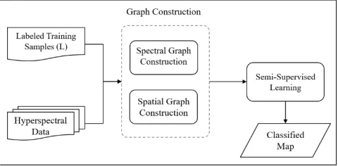
The proposed Spectral-Spatial GBSSL method consists of two steps, 1) two distinct spectral and spatial graphs are constructed to exploit the relationship among pixels in spectral and spatial spaces respectively, and then 2) the Laplacians of both constructed graphs are merged in order to form a weighted joint graph. Figure 1 illustrates the flowchart of the proposed framework.
2.1. Graph-based SSL
The graph-based is built based on the geometry of the whole data including both labeled and unlabeled ones. Each vertex of the graph is a data point, and edges represent the similarity between samples. The similarity between data points is calculated by RBF kernel of width σ:
= exp−‖� −� ‖2�2 2) (1)
To avoid self-similarity, is set to zero.
There are various methods to connect the vertices, in the fully-connected graph. Each data point is fully-connected to all the other samples. In the K-nearest neighbors graph method, two points will be connected, if one of them is among k-nearest neighbors of the other point. In this way, the affinity matrix is sparse, and computational advantages of sparse matrices can be utilized. In addition to the advantages such as speed and the required storage reduction, some studies have indicated that the sparse graphs can provide better modeling of manifold assumption (Chapelle, Schokopf, et al. 2006).
The main goal of graph-based SSL is finding a labeling function, which must be consistent with both the labels of initial training samples and the geometry of the whole data represented by graph structure.
Consistency with the initial labeled data can be calculated by:
∑�= � − = ‖��− ��‖ (2)
Where��= { , , … , �} is the l first labeled data, and ��is the predicted labels of these l samples by the labeling function. The equation (2) shows the empirical risk have to be minimized. But with the few labeled samples, the minimization problem will be ill-posed and the, solution would not be unique. Therefore, we need a regularization term limiting function space toprovide well-posed condition (Chapelle, Schokopf et al. 2006). On the other hand, consistency with the data geometry is motivated by smoothness assumption on the manifold. For this purpose, the labels of neighbor vertices should be close together, the difference between labels is given by:
Equation (3) will be used as the regularization term and states as much higher value of two points are more similar, and rapid changes in their labels is penalized severely.
The learning on the graph is performed by minimization of a quadratic cost function derived by combining empirical risk and the regularization term:
By solving the optimization problem (5), we will have the labeling function, �∗,as follows:
�∗= � + �� − �� (6)
Y is a n×c matrix where {� = | = , = , … , �}, and n is the number of labeled and unlabeled samples and c is the number of classes. The parameter � ∈ , is the weight of the Laplacian of the graph. The diagonal S n×n matrix is given by � = [�]�. To avoid singularity problem of Laplacian matrix and degenerate situation a small regularization term can also be added that has been called Tikhonov regularization (Tikhonov and Arsenin 1977).
�∗= � + �� + �� − �� (7)
The parameter μ is the Tikhonov regularization term which must be tuned appropriately.
2.2. Spatial-Spectral Graph Construction
As mentioned before, in this proposed method two graphs are constructed in order to address both spatial and spectral information. To construct the spectral graph, each pixel is connected to its K nearest neighbor pixels in spectral space. This implies smoothness assumption on the manifold where the close samples should have similar labels.
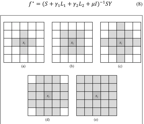
The spatial-based graph is constructed using computing spectral distance between each pixel and its spatial neighbors. Based on the size of the image, each pixel can be connected to L= 4, 8, 12, 20 and 24 spatial neighbors, the different spatial neighborhood definitions are illustrated in Figure 2 (a)-(e).
The spectral graph Laplacian (L1) and the spatial graph Laplacian (L2) are integrated by weighted summation and is replaced in (7), yields:
�∗= � + � � + � � + �� − �� (8)
In this way, the equation (8) guarantees the smoothness of labeling function on both spectral and spatial graphs simultaneously. The labeling function estimates the probability of a sample belonging to each class. At the end of the learning process, the predicted label of each sample is obtained as follows.
= max �( | ) = max � (9)
2.3. Speed-up Inversion Method
Although the spatial and spectral Laplacian matrices have large n×n size, they are sparse. This mainly because each graph have k×n edges and the affinity matrix has (k+1)×n non-zero elements. Although, � + � � + � � + �� is sparse, butnotnecessarily its inverse model. Therefore, calculating and storing of the inverse matrix induce a high computational complexity of O(n3) and O(n2) respectively. There is a need to utilize the high speed numerical methods in order to approximate the inverse of large sparse matrices accurately.
Conjugate Gradient (CG) method is the most distinguished iterative algorithm for solving sparse systems with too large size to be implemented by direct methods (Plaza and Chang 2007). To apply CG method on the linear equation� = , A must be a symmetric, positive definite and sparse matrix. Theoretically CG, method converges to the solution in n steps, but with good preconditioner choosing can get good approximation of solution in <<n steps (Fornasier, Peter et al. 2015).
3. EXPERIMENTAL RESULTS
3.1. Hyperspectral Data Sets
To evaluate the performance of our method, we used two different commonly used hyperspectral data sets with different spectral and spatial resolutions:
Indian Pines: the AVIRIS Indian Pine Image data set. This data set contains 145 by 145 pixels with 20m spatial resolution. The AVIRIS sensor provides 220 spectral bands
originally, but 35 bands include noisy and water absorption bands, and then are removed ([1-3], [103-112], [148-165], [217-220]), and finally, 185 bands are used in our experiments. There are 16 land cover classes in the scene with the size of 20 to 2468 pixels per class. The classes with size less than 100 pixels are removed, and 13 classes remain. The true color composite and the available labeled ground truth are presented in Figure 3 (a) and 3 (b) respectively.
(a) (b)
Figure 3. The 145×145 AVIRIS Indian Pine data set, (a) True color composite with bands R:26, G:14, B:8. (b)
Ground truth reference map.
Pavia University: This hyperspectral data set was acquired by Reflective Optics System Imaging Spectrometer (ROSIS) with 610 by 340 in size. The spatial and spectral resolutions provided by ROSIS sensor are 1.3 m and 115 bands respectively. Pavia University is an urban area with nine different classes with the size of 610×340 pixels. The high spatial resolution of ROSIS creates a challenging classification problem that our proposed method can appropriately handle. Figure 4 illustrates the true color composite of Pavia University and the available labeled ground truth.
(a) (b)
Figure 4. The 610×340 ROSIS Pavia University data set (a) True color composite with bands R:53, G:31, B:8. (b) Ground
truth reference map.
The hyperspectral data set is normalized by using: ̃ = /(√∑ ‖ ‖�
= ) (10)
Where xi is the spectral vector of each pixel.
3.2. Free Parameters Tuning Figure 2. The spatial-based graph construction using (a-e): 4,
Selecting the optimum values for free parameters is one of the most sensitive and time-consuming steps in SSL and have a serious influence on the method’s performance. In the proposed method, there are three continuous parameters� , � and µ indicate the weight of spectral, spatial graph and Tikhonov regularization term respectively. To optimize these parameters, grid search is implemented, which is an exhaustive search method. Before applying grid search, it is necessary to define a finite values for each parameter, we choose {0.05, 0.1, 0.15, … ,0.95} for search space.
3.3 Results
The proposed method is evaluated in ill-posed classification problem scenario where there is a very limited number of labeled samples compared to the high dimension of data. For Indian Pine data set, we used only {5, 10, 15, 30 and 50} labeled pixels per class and {5, 10, 15, 30, 50, 100} for ROSIS Pavia University as training set. To evaluate the classification performance for the classes with enough labeled samples, 350 sample per class were considered as a testing set. For the other classes, the rest of the labeled samples composed a testing set. The training and testing labeled samples are selected randomly using 10-fold cross-validation, and the results were reported as the Average Accuracy (AA).
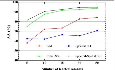
The superiority of our method was demonstrated in comparison with the state-of-the-art SVM method and graph-based SSL method using only spectral or spatial information. The optimum SVM parameters (C, γ) were also selected by grid search method. Figure 5. Illustrates the comparison of different methods with different labeled training size for AVIRIS Indian Pine data set. The same comparison results for Pavia University data are presented in Figure 6.
The effect of the number of used spatial and spectral neighbors are shown in Figure 7 and Figure 8 respectively. As shown in the results, we selected the best values as K=10 and L=8 to be employed in the proposed method for AVIRIS Indian Pine data set. Because of the different spatial resolution of Pavia University, these parameters were chosen as K=10 and L=12 to obtaining the maximum classification accuracy.
4. DISCUSSION
The parameter K is the number of used neighbors to construct a spectral graph. Figure 7 provides overall accuracy curves concerning the variation of K for different labeled training data sets. When K is too small, each vertex is connected to only a few similar pixels, and the classification performance is poor. When K increases to an optimum value equal to 5 or 10 for different training data sets, the classification accuracy is also increasing. Nonetheless, after this point, the performance remains unchanged or even degrades. Because when K becomes too large, the discriminative ability of the constructed graph decreases. The similar experimental results for the variation of spatial neighbors, (See Figure 8), confirmed the previous analysis. Therefore, by employing the best number of spectral and spatial neighbors the performance can be improved. The same analysis was done for the Pavia University data set, in order to select the optimum values and to construct the most discriminative graphs.
Figure 7. Classification performance of various spectral neighbors (K) with different size of labeled training samples in
AVIRIS Indian Pine data set
Figure 5. Classification performance of various methods with different size of labeled training samples in AVIRIS Indian
Pine data set.
Figure 6. Classification performance of various method with different size of labeled training samples in Pavia University
Figure 8. Classification performance of various spatial neighbors (L) with different size of labeled training samples in
AVIRIS Indian Pine data set
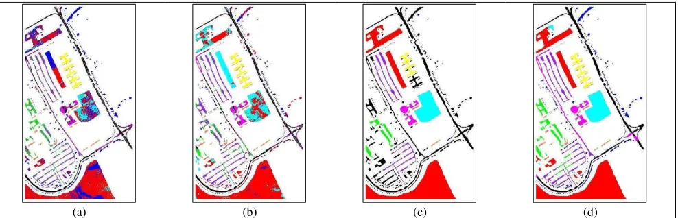
To demonstrate the effectiveness of the proposed method, we consider the worst scenario with only five labeled samples per class. The obtained classified maps by the proposed method and the baseline ones for AVIRIS Indian Pine and Pavia University data
sets are given in Figure 9 and Figure 10 respectively. As it can be seen, our method has the best performance in term of overall classification accuracy. Moreover, the classified maps consisting of homogeneous regions. In other words, employing the spatial information in graph construction provides the ability to solve classification and segmentation optimization problems simultaneously. Therefore the classes’ boundaries were extracted more precisely.
As shown in Figures 9(c) and 10(c), the spatial graph-based SSL results indicate that applying the spatial graph alone canalso ensure the smoothness of labeling function on the spectral graph and consequently achieves high classification performance. Although, the performance of SSL classification, by using only the spectral graph (Figure 9(b) and 10(b)) is not satisfactory. However, the contribution of both graphs to construct a joint Laplacian can improve the results. This improvement is more significant when the labeled training data set is too scarce, i.e. when there are only five labeled samples for each class. In this condition, the proposed method increases the classification accuracy by 5.92% and 10.76% compared to the spatial graph-based SSL for AVIRIS Indian Pine and Pavia University data sets respectively.
(a) (b) (c) (d)
Figure 9. Classification results on the AVIRIS Indian Pine data set, classification maps with five labeled samples per class using: (a) SVM method (OA=52.99%), (b) Spectral GBSSL (OA=57.4%), (c) Spatial GBSSL (OA=76.29%), (d) Spatial-Spectral GBSSL
(OA=82.8%).
(a) (b) (c) (d)
Figure 10. Classification results on the ROSIS Pavia University data set, classification maps with five labeled samples per class using: (a) SVM method (OA=68.41%), (b) Spectral GBSSL (OA=70.80%), (c) Spatial GBSSL (OA=79.21%), (d) Spatial-Spectral GBSSL
5. CONCLUSION
In this paper, we proposed a graph-based semi-supervised learning algorithm which uses both spectral and spatial information to construct the graph Laplacian. Experimental results from the AVIRIS Indian Pine and the ROSIS Pavia University data sets showed the superiority of the proposed method over the supervised SVM classifier. In addition, compared to SSL methods using only a single spectral/spatial graph, the proposed framework of spectral-spatial SSL method improved the classification performance. As shown in the numerical results, when the number of labeled training samples was very limited, the proposed method had the largest increase in the classification accuracy. In other words, the proposed spectral-spatial SSL method was able to efficiently overcome the Hughes phenomena and also had an outstanding performance.
6. REFERENCES
Camps-Valls, G., et al. (2007). "Semi-supervised graph-based hyperspectral image classification." Geoscience and Remote Sensing, IEEE Transactions on 45(10): 3044-3054.
Chapelle, O., et al. (2006). Semi-supervised learning (Adaptive Computation and Machine Learning). Massachusetts, The MIT press.
Chen, Z. and B. Wang (2016). "Spectral-Spatial Classification Based on Affinity Scoring for Hyperspectral Imagery." IEEE Journal of Selected Topics in Applied Earth Observations and Remote Sensing 9(6): 2305-2320.
Fauvel, M., et al. (2015). "Fast Forward Feature Selection of Hyperspectral Images for Classification With Gaussian Mixture Models." Selected Topics in Applied Earth Observations and Remote Sensing, IEEE Journal of 8(6): 2824-2831.
Fornasier, M., et al. (2015). "Conjugate gradient acceleration of iteratively re-weighted least squares methods." arXiv preprint arXiv:1509.04063.
Jia, X., et al. (2013). "Feature mining for hyperspectral image classification." Proceedings of the IEEE 101(3): 676-697.
Li, J., et al. (2010). "Semisupervised hyperspectral image segmentation using multinomial logistic regression with active learning." Geoscience and Remote Sensing, IEEE Transactions on 48(11): 4085-4098.
Liu, Z., et al. (2017). "Class-Specific Random Forest With Cross-Correlation Constraints for Spectral-Spatial Hyperspectral Image Classification." IEEE Geoscience and Remote Sensing Letters PP(99): 1-5.
Ma, L., et al. (2015). "Local-Manifold-Learning-Based Graph Construction for Semisupervised Hyperspectral Image Classification." IEEE transactions on Geoscience and Remote Sensing 53(5): 2832-2844.
Persello, C. and L. Bruzzone (2014). "Active and semisupervised learning for the classification of remote sensing images." Geoscience and Remote Sensing, IEEE Transactions on 52(11): 6937-6956.
Plaza, A. J., and C.-I. Chang (2007). High-performance computing in remote sensing, CRC Press.
Shahshahani, B. M. and D. A. Landgrebe (1994). "The effect of unlabeled samples in reducing the small sample size problem and mitigating the Hughes phenomenon." IEEE Transactions on Geoscience and Remote Sensing 32(5): 1087-1095.
Tikhonov, A. N., and V. I. A. k. Arsenin (1977). Solutions of ill-posed problems, Vh Winston.
Tuia, D., et al. (2010). "A survey of active learning algorithms for supervised remote sensing image classification." Selected Topics in Signal Processing, IEEE Journal of 5(3): 606-617.
Zhang, Q., et al. (2015). "Automatic spatial–spectral feature selection for the hyperspectral image via discriminative sparse multimodal learning." Geoscience and Remote Sensing, IEEE Transactions on 53(1): 261-279.