Full Terms & Conditions of access and use can be found at
http://www.tandfonline.com/action/journalInformation?journalCode=ubes20
Download by: [Universitas Maritim Raja Ali Haji] Date: 11 January 2016, At: 19:32
Journal of Business & Economic Statistics
ISSN: 0735-0015 (Print) 1537-2707 (Online) Journal homepage: http://www.tandfonline.com/loi/ubes20
Inference for Local Autocorrelations in Locally
Stationary Models
Zhibiao Zhao
To cite this article: Zhibiao Zhao (2015) Inference for Local Autocorrelations in Locally Stationary Models, Journal of Business & Economic Statistics, 33:2, 296-306, DOI: 10.1080/07350015.2014.948177
To link to this article: http://dx.doi.org/10.1080/07350015.2014.948177
Accepted author version posted online: 08 Aug 2014.
Submit your article to this journal
Article views: 150
View related articles
Inference for Local Autocorrelations in Locally
Stationary Models
Zhibiao Z
HAODepartment of Statistics, Penn State University, University Park, PA 16802 ([email protected])
For nonstationary processes, the time-varying correlation structure provides useful insights into the un-derlying model dynamics. We study estimation and inferences for local autocorrelation process in locally stationary time series. Our constructed simultaneous confidence band can be used to address important hypothesis testing problems, such as whether the local autocorrelation process is indeed time-varying and whether the local autocorrelation is zero. In particular, our result provides an important generalization of the R functionacf()to locally stationary Gaussian processes. Simulation studies and two empirical applications are developed. For the global temperature series, we find that the local autocorrelations are time-varying and have a “V” shape during 1910–1960. For the S&P 500 index, we conclude that the returns satisfy the efficient-market hypothesis whereas the magnitudes of returns show significant local autocorrelations.
KEYWORDS: Nonparametric regression; Simultaneous confidence band; Testing for zero autocorrela-tion; Time series.
1. INTRODUCTION
Practical data often exhibit complicated time-varying pat-terns that can hardly be captured by simple parametric models, such as the classical autoregressive moving average models. To model nonstationary data, locally stationary models allow the model dynamics to change smoothly in time and thus can provide flexible and tractable alternatives over stationary mod-els. Using spectral representations, Dahlhaus (1997) and Adak (1998) studied locally stationary models; other related works in-clude Priestley (1965) and Ombao, Von Sachs, and Guo (2005). In time domain analysis, Subba Rao (1970) proposed time-varying autoregressive models, Davis, Lee, and Rodriguez-Yam (2006) studied piecewise stationary autoregressive models, and Dahlhaus and Subba Rao (2006) considered time-varying au-toregressive conditional heteroscedastic (ARCH) models. For locally stationary wavelet processes, see Nason, Von Sachs, and Kroisandt (2000) and Van Bellegem and Von Sachs (2008). See Dahlhaus (2012) for a survey of contributions.
For nonstationary data, the time-varying dependence/ correlation structure can provide useful insights into the dy-namics of the underlying process, such as whether and how the dependence changes over time. For example, in global tempera-ture studies, it is of interest to examine whether the dependence of temperature measurements has changed over the past cen-tury. In children’s growth studies, it is reasonable to believe that the dependence of growth measurements has different patterns during early childhood, middle childhood, and adolescence. In financial markets, we can ask whether the market returns are more correlated in periods with high volatilities. In these ap-plications, one common feature is the potentially time-varying dependence/correlation structure, and traditional tools based on the autocorrelations of stationary processes are of little use.
Motivated by the above discussion, we aim to study autocorre-lations of locally stationary processes. For stationary processes, there is a vast literature on autocovariances/autocorrelations; see Wu and Xiao (2012) for a survey. On the other hand, devel-opments on autocovariances/autocorrelations of nonstationary
processes are quite limited. One approach is to divide data into blockwise stationary models (Ombao et al.2001; Davis, Lee, and Rodriguez-Yam2006), but this approach relies on selecting the number, location, and length of the blocks. For autocovari-ance estimation of locally stationary processes, some alterna-tive approaches include the local cosine function method in Mallat, Papanicolaou, and Zhang (1998), the wavelet peri-odograms method in Nason, Von Sachs, and Kroisandt (2000), and the local kernel autocovariance estimation in Dahlhaus (2012). However, these works did not obtain the related point-wise and simultaneous asymptotic distributions, the essential ingredients in statistical inference.
Our first goal is to quantify and estimate the time-varying correlation structure for a rich class of locally stationary time series introduced in Wu and Zhou (2011). At each lagk, we in-troduce the local autocorrelation curve, denoted by{ρk(t)}t∈(0,1), to characterize the local correlation of measurements near time t∈(0,1). As a time-varying curve, the local autocorrelation curve is a natural generalization of the classical autocorrelation function for stationary processes to locally stationary processes. Using the nonparametric kernel smoothing method, we propose a local sample autocorrelation estimate ofρk(t).
Our second goal is to construct a simultaneous confidence band (SCB) for{ρk(t)}t∈(0,1). Compared to a pointwise confi-dence interval, an SCB can provide more useful insights into the overall trend ofρk(t) on the time intervalt ∈(0,1). In the literature, SCB has been constructed for various marginal char-acteristics, including the marginal density function (Bickel and Rosenblatt1973), nonparametric mean function (Eubank and Speckman1993; Wu and Zhao2007), and coefficient functions in varying-coefficient linear models (Fan and Zhang 2000).
© 2015American Statistical Association Journal of Business & Economic Statistics
April 2015, Vol. 33, No. 2 DOI:10.1080/07350015.2014.948177
Color versions of one or more of the figures in the article can be found online atwww.tandfonline.com/r/jbes.
296
1850 1900 1950 2000
−1.0
−0.5
0.0
0
.5
Time (year)
T
e
mper
ature Anomalies (Celsius)
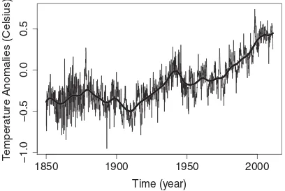
Figure 1. The global monthly temperature anomalies in Celsius during 1850–2010, and the local linear estimate of the mean trend (thick solid curve).
These marginal quantities are less informative when the goal is to study how time series observations are correlated with each other.
Our development on SCB for {ρk(t)}t∈(0,1) provides an ap-pealing tool for a nonparametric assessment of the time-varying dynamics of the underlying model. The constructed nonpara-metric SCB can be used to examine whether the local auto-correlation curve is of certain parametric patterns by checking whether the parametric curve is contained within the SCB. We develop easy-to-use rule-of-thumb tests for some practically important hypotheses: (i) whether the local autocorrelations are indeed time-varying or constant, and (ii) whether the local auto-correlations are significant or not. For stationary time series, the R functionacf()plots sample autocorrelations along with two horizontal 95% critical lines to examine whether there are sig-nificant autocorrelations among observations. By constructing the 95% simultaneous cutoff bands, we provide an important generalization of the latter result to local autocorrelations of locally stationary processes.
The developed methodology for local autocorrelations has a wide range of applications in social and scientific fields, such as biomedical, climatic, environmental, economics, and financial fields, where nonstationary processes occur frequently. In Sec-tion6, we illustrate two applications in the global temperature series and the S&P 500 index, and our methodology yields some interesting findings.
2. TWO MOTIVATING DATASETS
2.1 Global Temperature Series
Consider the global monthly temperature anomalies dur-ing 1850–2010, relative to the 1961–1990 mean. The con-tinually updated dataset is available at http://cdiac.ornl.gov/ ftp/trends/temp/jonescru/global.txt,and detailed background in-formation can be found at http://cdiac.ornl.gov/trends/temp/ jonescru/jones.html.
There are n=161∗12=1932 observations, with a time series plot inFigure 1.
Figure 1clearly indicates a time-varying trend, and in cli-mate change studies there is a substantial literature on infer-ences for the mean trend μ(t). For example, Woodward and
Gray (1993) fitted a linear trend, Rust (2003) argued that a linear trend is inadequate and fitted a quadratic trend, Wu, Woodroofe, and Mentz (2001) considered an isotonic regres-sion to examine the change point in the mean trend, and Wu and Zhao (2007) constructed a simultaneous confidence band for the mean trend. The thick solid curve inFigure 1is the non-parametric smoothing estimate ofμ(t); see Section6.1for more details.
While the aforementioned works provided an extensive ac-count of inferences for the mean trendμ(t), there are two limi-tations. First, they all assumed that the temperature series has a mean trend plus some stationary errors. As a modeling issue, it is hard to justify that the mean is time-varying while the depen-dence structure of the errors remains the same over the long time period of 161 years. In fact, our methodology (see Section6.1) suggests that the error process has a complicated time-varying pattern, and thus the stationarity-based inference may be ques-tionable. Second, these works did not address the equally im-portant question of whether and how the dependence structure of temperature series varies over time. In contrast to the first-order marginal mean trend, the autocovariance/autocorrelation concerns the second-order property of the temperature series and can provide useful insights into the evolving dynamics of the series.
2.2 S&P 500 Index Returns
In finance, the efficient-market hypothesis (EMH) states that financial markets are efficient: stock price behaves like ran-dom walks and all subsequent price changes represent ranran-dom departures from previous prices. See the review article Fama (1970). In terms of autocorrelations, EMH asserts that stock returns have zero autocorrelations and thus are not predictable. On the other hand, however, there is empirical evidence (Ding et al.1993) that the absolute values or magnitudes of returns are correlated.
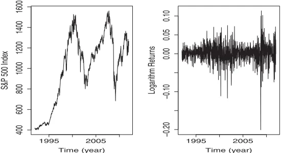
The S&P 500 index includes 500 large-cap companies in lead-ing industries of the U.S. economy and is one of the most widely used benchmarks for the overall U.S. stock market performance. Since weekly data are less noisy/volatile than daily data, we consider the weekly S&P 500 index during the 20 years period January 6, 1992–December 27, 2011; see the left plot in Fig-ure 2. Denote the logarithm returns byXi=log(Si)−log(Si−1), where Si is the index at weeki. There aren=1041 observa-tions, plotted in the right plot of Figure 2. It is desirable to develop some test for the EMH that can work under possible time-varying dependence of unknown form.
3. INFERENCES FOR LOCAL AUTOCORRELATION
CURVE
Motivated by the two examples in Section2, in this section we study the time-varying dependence structure of nonstationary processes. For a random variableZ, write Z∈Lq if
Zq := [E(|Z|q)]1/q<
∞, q >0.
1995 2005
400
600
800
1000
1200
1400
1600
Time (year)
S&P 500 Inde
x
1995 2005
−0.20
−0.10
0.00
0.05
0.10
Time (year)
Logar
ithm Retur
ns
Figure 2. Weekly S&P 500 index (left plot) and logarithm returns (right plot) during 1992–2011.
3.1 Local Autocorrelation Curve
We consider the nonstationary time series in Wu and Zhou (2011):
Xi =g(ti, ξi), where ti =i/n, ξi=(. . . , εi−1, εi),
i=1, . . . , n, (1)
for iid innovations {εi} and a time-varying transformation g(ti,·). Assume
sup
t
g(t, ξ0)2 <∞ and
lim sup |t−s|→0
g(t, ξ0)−g(s, ξ0)2=0. (2)
ThenXi =g(ti, ξi)=g(t, ξi)+op(1) forti≈t. That is, in the local time window ti≈t,{Xi}i can be approximated by the stationary process {g(t, ξi)}i. Following Dahlhaus (1997) and Wu and Zhou (2011), we say that{Xi}i is locally stationary. Therefore, (1) allows the dependence structure to vary over time, and meanwhile it imposes a local stationarity. In time series analysis, autocorrelation functions measure the strength of dependence in a process. The autocorrelation functionρ(·,·) for{Xi}at lagk≥0 is
ρ(i, k)= √ γ(i, i+k)
γ(i, i)γ(i+k, i+k), where
γ(i, i+k)=cov(Xi, Xi+k). (3)
By stationarity of ξi, γ(i, i+k)=cov{g(ti, ξ0), g(ti+k, ξk)}. Lett ∈(0,1) be any fixed time point. Consideri= ⌊nt⌋, with
⌊x⌋being the integer part ofx, so thatti = ⌊nt⌋/n→tasn→
∞. Letkbe fixed. Usingg(ti, ξ0)g(ti+k, ξk)−g(t, ξ0)g(t, ξk)=
{g(ti, ξ0)−g(t, ξ0)}g(ti+k, ξk)+ {g(ti+k, ξk)−g(t, ξk)}g(t, ξ0) and the inequality E|U V| ≤ U2V2, we obtain the following result:
Proposition 1. Suppose (2) holds. Then for any fixedk≥0 andt∈(0,1),
lim
n→∞ρ(⌊nt⌋, k)= γk(t) γ0(t)
def
=ρk(t), where
γk(t)=cov{g(t, ξ0), g(t, ξk)}. (4)
Ifg(t, ξi) does not depend ont, thenρk(t) is a constant and reduces to the usual autocorrelation function for stationary pro-cesses. In our locally stationary case, the time-varying curve ρk(t) measures the correlation of observations in a neighbor-hood oft. We call{ρk(t)}t∈[0,1]the local autocorrelation curve.
Example 1. Consider the fixed-design nonparametric regres-sion model: Xi =μ(ti)+σ(ti)ei, i=1, . . . , n, where {ei ∈
L2
}i∈Zis a centered stationary process,μ(t) andσ(t) are con-tinuous functions on [0,1] representing the time-varying trend and scale, respectively. Thenρk(t)=corr(e0, ek) is a constant, although the variance changes over time.
Example 2. The classical linear process isei =∞j=0αjεi−j, where {εi∈L2
}i∈Z are iid random variables with E(εi)=0, and{αj}j≥0are constants satisfying∞j=0α
2
j <∞. For a natu-ral extension, we consider the linear process with time-varying coefficients:
ei(t)=
∞
j=0
αj(t)εi−j, i∈Z, t ∈[0,1], (5)
whereαj(t), j ≥0,are continuous functions on [0,1] satisfying supt∈[0,1]
∞
j=0α 2
j(t)<∞. LetXi =ei(ti) be discrete samples. Thenρk(t)=∞j=0αj(t)αj+k(t)/∞j=0α
2
j(t). Ifαj(t)=0 for j ≥q+1, then (5) is the time-varying coefficient moving average of orderq. Consider the time-varying autoregressive model:ei(t)=α(t)ei−1(t)+σ(t)εi for some continuous func-tionsα(t) andσ(t) on [0,1]. Note that this is different from the time-varying autoregressive model ei =α(i/n)ei+σ(i/n)εi in, for example, Subba Rao (1970), which does not admit the representation (5). If supt∈[0,1]|α(t)|<1, then (5) holds with
αj(t)=σ(t)αj(t) andρk(t)=αk(t).
Example 3. Consider the threshold autoregressive model ei =α|ei−1| +
√
1−α2εi, where
{εi}are iid N(0,1) random variables, andα∈(−1,1) controls the dependence. By Andel, Netuka, and Svara (1984), the stationary distribution has the skew-normal density f(u)=2φ(u) (αu/√1−α2), where φ and are the standard normal density and distribution functions, respectively. We consider the extension to the time-varying
coefficient case:
Example 4. In econometrics, the widely used GARCH(1,1) model is ei =σiεi, σi2=α0+α1e2i−1+βσ
2
i−1, where α0> 0, α1≥0, β≥0, and{εi}are iid noises with zero mean and unit variance. As in Examples 2–3, the corresponding time-varying coefficient GARCH(1,1) is ei(t)=σi(t)εi, σi2(t)=α0(t)+
α1(t)ei2−1(t)+β(t)σi2−1(t), i ∈Z, t∈[0,1], where α0(t)>0 andα1(t)≥0, β(t)≥0 are continuous functions on [0,1] sat-isfying inftα0(t)>0 and supt[α1(t)+β(t)]<1. As a special case, if β(t)=0, then the latter model reduces to the time-varying coefficient ARCH(1) model in Dahlhaus and Subba Rao (2006). LetXi =ei(ti) be discrete samples. Thenρk(t)=0 for k≥1.
3.2 Local Sample Autocorrelation Process
Throughout this article, our theory and methods rely on the assumptionμ(t) :=E[g(t, ξ0)]=0 for alltso thatE(Xi)=0. In practice, we can subtract a nonparametric estimate ofμ(ti) fromXi; see Section6.1. Due to technical difficulty, it is non-trivial to theoretically quantify the impact from precentering the data. From our simulation study in Section5, our methods still yield reasonable performance when we precenter the data us-ing local linear regression. Based on our empirical studies, we recommend:
(i) For time series data (e.g., global temperature series) with a clear time trend, use the local linear regression to remove the trend; see Section6.1.
(ii) For daily or weekly financial returns data, the returns usu-ally oscillate around zero and are negligible relative to the volatility, and thus we can assume that the returns are al-ready centered. For absolute returns, we can use the local linear regression to remove the trend. For squared returns, the time trend is usually negligible (for a 1% return, the squared return is 0.0001) relative to the strength of the autocorrelation and the potential error from fitting a com-plicated local linear regression, and thus we recommend simply subtracting the sample mean squared returns.
GivenX1, . . . , Xn from (1), we discuss estimation of ρk(t) at a given t ∈(0,1). If {Xi} is stationary, then ρk(t) is a constant and can be estimated by the sample correlation
0.0 0.2 0.4 0.6 0.8 1.0
(7). The solid, dotted, dashed, and dot-dashed curves correspond to
α(t)=0.5, 0.9t, 0.9 sin(π t), and 2φ(t−0.3), respectively.
(n−1n−k
i=1XiXi+k)/(n−1ni=1X 2
i). For (1), in light of the lo-cal stationarity, we propose estimatingρk(t) based on local data withti ≈t. Specifically, we propose the following nonparamet-ric kernel smoothing estimate: is the sample autocorrelation based on local data, we call
{ρkˆ (t)}t∈(0,1)the local sample autocorrelation process.
In (1), the pair (g, ξi) determines the probabilistic structure of
{Xi}. To study asymptotic properties, we impose the following dependence condition:
Assumption 1. For p, q >0, we write (g, ξi)∈SLC(p )-GMC(q) if they satisfy Lp stochastic Lipschitz continu-ity (SLC) condition and Lq geometric moment contrac-tion (GMC) condicontrac-tion in the sense: (i) sups=tg(t, ξ0)−
Assumption 1(i) imposes a stochastic (Lp
norm) Lips-chitz continuity condition on g as inferences would be im-possible if data jump randomly without any continuity. In (9), supt∈[0,1]g(t, ξ0)q <∞ imposes the finite qth moment
assumption, andωi measures the effect of replacingε0with an iid copy ε′
0, which in turn imposes explicit conditions on the strength of the dependence. Assumption 1 is satisfied for many linear and nonlinear locally stationary time series; see Wu and Zhou (2011).
Assumption 2.(i)K(·) has support [−1,1], is symmetric and continuously differentiable, and RK(u)du=1; throughout, ψK =Ru2K(u)du/2, ϕK =RK2(u)du. (ii) nb9logn→0 andnb2/(logn)8
→ ∞. (iii)γk(t) andγ0(t) are four times con-tinuously differentiable.
Theorem 1. Let (g, ξi)∈SLC(4)-GMC(8) (see Assumption 1) and Assumption 2 hold. Defineβi,k(t)=[g(t, ξi)g(t, ξi+k)−
It is worth pointing out that the fourth differentiability onγk(t) in Assumption 2 (iii) can be weakened to twice differentiability under a stronger bandwidth condition.
3.3 Simultaneous Confidence Band
Theorem 1 can be used to construct an asymptotic pointwise confidence interval forρk(t) at eacht∈[b,1−b]. However, in practice, it is desirable to construct a simultaneous confidence band (SCB). We say that [l(t), u(t)] is an asymptotic (1−α)
Theorem 2. Assume the same conditions in Theorem 1. Then, for allz∈R,
The limiting distribution in (12) is the extreme value distri-bution. In Section3.4, we show that the biasb2ψKλ(t) can be reduced to a negligible high-order term by using a higher-order kernel. Therefore, let ˆŴk(t) be a consistent estimate ofŴk(t) (see
The factorC(b, α) reflects the simultaneousness of the confi-dence band. By contrast, if we replaceC(b, α) in (12) by the (1−α/2) standard normal quantile, by Theorem 1, then we have a pointwise (1−α) confidence band. In practice, SCB can depict the overall trend and variability of the processρk(t); see Sections4.2and4.3for applications of SCB.
3.4 Bandwidth Selection and Bias Correction
Bandwidth selection:The estimator ˆγk(t) in (8) is the Priest-ley and Chao (1972) nonparametric kernel smoothing esti-mator of the mean trend cov(Xi, Xi+k) in the fixed-design regressionXiXi+k=cov(Xi, Xi+k)+e∗i withe∗i =XiXi+k− cov(Xi, Xi+k). For nonparametric regression of independent data, Ruppert, Sheather, and Wand (1995) proposed an auto-matic bandwidth selector, which is well-known to undersmooth correlated data. Letb∗be the automatic bandwidth implemented using the function dpill in the R package KernSmooth. Based on our simulations in Section5,b=1.5b∗works quite well. To avoid choosingb for eachk, we choose b based on k=0 and use the samebfor allk.
Bias correction:In Theorems 1–2, due to the unknown deriva-tives γ′′ out that using this higher-order kernel does not completely re-move the bias, instead there are still negligible higher-order bias terms of the orderO(b4).
4. GAUSSIANITY-BASED RULE-OF-THUMB
INFERENCES
In this section, we assume that{g(t, ξi)}i∈Z is a Gaussian process for each t and develop some easy-to-use inferences, which we term by the rule-of-thumb inferences.
While it may seem restrictive at first, the Gaussian assumption is quite reasonable here based on two facts: (i) by the Wold’s de-composition, any zero-mean covariance-stationary process can be represented by a linear process with uncorrelated innovations (assuming no deterministic component); and (ii) Gaussian pro-cess and linear propro-cesses with independent innovations share the equivalent second-order moment properties. Thus, in light of the local stationarity of the locally stationary process, to study our (second-order) local autocorrelations, it is reasonable to work under the locally stationary Gaussian framework, provided that we ignore the gap between the uncorrelation and independence in the aforementioned (i) and (ii). In fact, in the literature on locally stationary processes, the Gaussian assumption is fre-quently imposed to facilitate inferences (Nason, Von Sachs, and
Kroisandt2000; Van Bellegem and Von Sachs2008). Further-more, simulation studies in Section 5 show that the rule-of-thumb inferences work reasonably well even for non-Gaussian processes.
4.1 Rule-of-Thumb Estimation ofŴ2k(t) and
Rule-of-Thumb SCB
To implement the SCB in Section3.3, we need to estimate the long-run varianceŴ2
k(t) in (10). For stationary processes, long-run variance estimation involves the selection of a block length parameter and has the optimal convergence rateO(n1/3) (Lahiri
2003). For locally stationary processes, this problem becomes even more challenging as we can only use local data, and as a result we need to choose both a block length parameter and a local bandwidth, and the convergence rate of the estimator can be quite slow. To attenuate these issues, we propose a rule-of-thumb estimator based on the Gaussian assumption.
Proposition 2. Suppose{g(t, ξi)}i∈Z is a Gaussian process. extra estimation. However, it is nontrivial to chooseL. For sta-tionary processes, the optimalL∝n1/3. In our locally stationary case, the optimal bandwidthb∝n−1/5and the local sample size
∝n4/5, thus we proposeL
=̺(n4/5)1/3
=̺n4/15 for some̺. By our simulations,̺=2 performs well.
Substituting the rule-of-thumb estimator ˆŴ2
k(t) in (14) into (12), we obtain the rule-of-thumb SCB. With the given kernel in Section3.4, the 1−α=95% SCB in (12) becomes
4.2 Test for Constant or Zero Local Autocorrelations at
a Given Lag
Nonparametric SCB for{ρk(t)}offers a reference to which other parametric autocorrelations can compare. By examining whether the parametric autocorrelation is contained within the 95% SCB (15), we can decide whether to reject a parametric null hypothesis at significance level 5%. This and next sections address some important hypotheses.
and check whether ˆρkis contained within the SCB.
Another interesting question is to test H0 : ρk(t)=0, t∈ [0,1],at a given lagk. We can examine whether the constant horizontal lineρk(t)=0 is contained within the SCB.
4.3 Test for Local Uncorrelation: An Extension of R
Functionacf()
In R, the functionacf()computes the sample autocorrela-tions along with two horizontal dashed blue lines±1.96/√n, which are the 95% acceptance region for the null hypothesis of zero autocorrelations based on the assumption ofniid normal random variables. Any significant departure from the two lines would indicate significant autocorrelations. We shall develop a counterpart result for local autocorrelations of locally stationary processes.
As in R, we assume that{g(t, ξi)}i∈Zis a Gaussian process for eacht. We are interested in the null hypothesis of zero local autocorrelations at all lags (or local uncorrelation):
H0:ρk(t)=0, t∈[0,1], duced by acf()for stationary processes. In our locally sta-tionary case,nb/ϕK reflects the effective local sample size, and C(b, α) is from the simultaneousness of the bands. In practice, we use 1−α=95% and the kernelK(·) given in Section3.4,
The bands (19) are model-free, easy to implement, and can serve as a rule-of-thumb criterion for testing for zero autocorre-lations of locally stationary Gaussian processes. Any significant departure from the bands would suggest rejection of the null hypothesis.
Remark 1. We can apply the above method to test for lo-cal uncorrelation of residuals from parametric models. Con-siderXi =μ(θ, Ui)+ei, whereUiis the covariate,μ(θ,·) is a parametric function with unknown parameter vectorθ, and{ei} is a locally stationary process. For example, μ(θ, Ui)=θTUi corresponds to the linear model. Let ˆθ be a√n-consistent es-timate of θ. Suppose each component of the partial deriva-tive ∂μ(θ, Ui)/∂θ can be bounded by some random variable L(Ui)∈L2
uniformly in iand a neighborhood of θ. Since ˆθ has a faster parametric convergence rate (√n) than the nonpara-metric rate (√nb) of the local sample autocorrelation, it can be shown that the impact from estimatingθ is negligible and thus the method can be used to test for local uncorrelation of{eˆi}.
Table 1. Empirical coverage probability and power for Models 1–3 in (20)–(22). Columns 90% and 95% are the empirical coverage probabilities when the nominal levels are 90% and 95%, respectively. ColumnsH1
0 andH 2
0 are the empirical power for testing the two null
hypotheses in (23) with significance level 5%. In (14), we useL=10≈2n4/15
b=b∗ b=1.5b∗ b=2b∗
ρ1(·) ρ2(·) ρ1(·) ρ2(·) ρ1(·) ρ2(·) θ b∗ 90% 95% H1
0 90% 95% H02 90% 95% H01 90% 95% H02 90% 95% H01 90% 95% H02
(a) Model 1 in (20)
0.0 0.065 91.1 95.0 4.5 91.9 96.3 100 90.1 95.4 4.7 90.1 94.7 100 88.6 95.5 5.4 88.8 94.4 100 0.2 0.059 89.9 94.3 77.3 91.5 95.6 100 90.8 95.0 89.1 90.9 95.9 100 90.4 95.3 94.9 89.5 95.5 100 0.5 0.051 90.7 95.8 100 89.1 93.2 99.8 90.8 95.7 100 89.9 94.8 100 89.2 94.9 100 89.6 94.0 100 0.8 0.056 92.7 97.3 100 89.7 93.6 98.6 90.6 96.4 100 88.7 94.8 99.7 89.7 95.4 100 87.1 94.4 99.8 1.0 0.061 92.1 96.0 99.9 89.1 93.9 98.2 90.5 95.5 100 89.0 94.2 99.7 87.6 94.4 100 88.0 94.9 100
(b) Model 2 in (21)
0.0 0.043 90.8 94.9 2.7 86.4 91.4 6.2 90.8 95.3 2.2 89.1 94.2 3.7 91.9 95.6 1.4 89.4 95.1 2.3 0.2 0.058 92.1 97.2 11.2 88.7 94.1 10.4 91.2 96.0 11.6 89.8 94.6 10.3 91.2 96.1 13.8 90.9 95.2 10.9 0.5 0.064 92.2 97.3 79.1 91.2 95.7 21.8 90.7 96.1 89.2 89.6 95.9 28.5 85.6 94.4 93.7 87.2 93.5 33.0 0.8 0.062 91.9 95.8 99.9 90.6 95.4 14.8 90.9 95.4 100 89.0 94.4 15.7 81.6 91.4 100 80.9 89.6 13.6 1.0 0.051 92.2 96.1 100 88.7 93.3 14.9 88.9 95.7 100 87.6 93.4 16.4 83.6 91.3 100 80.5 89.5 12.6
(c) Model 3 in (22), centered using the theoretical mean
0.0 0.094 92.8 95.9 1.5 93.4 97.0 0.8 90.4 95.6 1.4 90.6 96.1 0.8 89.0 95.1 1.2 88.9 95.2 0.9 0.2 0.094 93.3 96.8 1.1 94.2 97.2 0.5 90.1 95.9 1.5 91.2 96.6 0.4 87.9 94.5 1.1 89.5 95.9 0.6 0.5 0.091 92.4 96.9 2.3 93.1 97.3 1.4 90.9 95.8 2.6 91.3 96.2 0.9 88.2 94.9 4.3 89.1 95.1 0.9 0.8 0.084 90.3 95.3 21.7 92.5 96.3 3.5 89.1 94.8 31.3 90.3 95.3 4.0 86.0 93.7 37.9 87.4 94.7 3.7 1.0 0.077 85.7 91.8 71.0 89.7 94.5 22.4 84.9 91.5 83.0 85.7 92.7 30.3 76.1 87.6 88.2 79.8 89.0 35.0
(d) Model 3 in (22), centered using local linear regression
0.0 0.094 92.0 96.4 0.5 93.9 97.6 0.9 90.1 94.6 1.0 91.5 96.1 1.0 88.1 93.7 1.1 88.5 95.5 1.0 0.2 0.094 90.8 96.4 1.4 92.9 96.5 0.9 88.1 93.7 1.3 90.9 95.2 0.9 88.2 93.6 1.3 88.7 94.4 0.6 0.5 0.089 90.8 96.7 2.7 92.6 96.6 1.6 88.7 95.3 3.2 89.9 95.9 1.3 85.9 93.7 3.6 88.0 95.2 1.1 0.8 0.086 87.7 93.2 22.0 90.2 94.7 3.1 83.9 91.3 31.8 86.5 92.7 3.7 79.4 87.9 37.7 82.0 90.4 4.8 1.0 0.082 83.0 90.4 72.4 81.5 89.0 19.6 75.8 85.1 82.1 75.3 84.7 25.3 65.8 76.8 86.4 63.2 75.1 30.0
Remark 2. To test for uncorrelation of stationary process, the cutoff lines±1.96/√n work for a given lag, and we can use some portmanteau test, such as the Ljung–Box test, to combine autocorrelations at multiple lags. Our SCB is simultaneous with respect to the timetbut for a given lagk, and it seems quite chal-lenging to extend the Ljung–Box test to our local autocorrelation setting. This will serve as a direction for future research.
5. SIMULATION STUDIES
Consider Xi =ei(ti), i=1, . . . , n, where {ei(ti)}i are dis-crete samples from a process{ei(t)}i. Let{εi}be iid standard normal variables. Consider three models for{ei(t)}:
Model 1: ei(t)=εi+3θ t εi−1−cos(π t)εi−2, (20) Model 2: ei(t)=0.6{(1−θ)+θsin(2π t)}ei−1(t)+εi,
(21)
Model 3: ei(t)=0.9θ t|ei−1(t)| +
1−(0.9θ t)2εi. (22)
Here the parameter θ ∈[0,1] controls the strength of the dependence and the shape of local autocorrelations. Models 1 and 2 are special cases of Example 2 and Model 3 is a special case of Example 3. Due to nonlinearity, Model 3 is a non-Gaussian process. We use Model 3 to examine the impact from
precentering the data. Specifically, we consider two approaches: (i) subtract the theoretical mean 0.9θ ti√2/π fromXi; and (ii) subtract the estimated mean using the local linear regression (24) in Section6.1.
For each choice of θ=0.0,0.2,0.5,0.8,1.0, we examine the empirical coverage probabilities of the constructed SCBs for{ρ1(t)}t∈[0.1,0.9]and{ρ2(t)}t∈[0.1,0.9]and the power of the test based on SCB. For the empirical coverage probabilities, two nominal levels 90% and 95% are considered. For SCB-based tests in Section4, we consider the null hypotheses:
H0k:ρk(t), t ∈[0.1,0.9], is a constant function, k=1,2, (23)
for each of the three models with significance level 5%. To ex-amine the effect of the bandwidthb, following the discussion in Section3.4, we use three choicesb=b∗,1.5b∗,2b∗, where b∗(the second column ofTable 1) is the average of 1000 band-widths based on the automatic bandwidth selector implemented using the R command dpill. In all cases, we use sample sizen=500 and compute the coverage probabilities and power based on 1000 realizations. As discussed in Section4.1, we use L=10≈2n4/15in (14).
The results are summarized inTable 1. Overall, the empir-ical coverage probabilities are close to the two nominal levels
1850 1900 1950 2000
−0.2
0.0
0.2
0.4
0.6
0.8
1.0
Time (year)
Local Sample A
utocorrelation Process
1850 1900 1950 2000
−0.2
0.0
0.2
0.4
0.6
0.8
1.0
Time (year)
SCB f
or Local A
utocorrelation at Lag 1
1850 1900 1950 2000
−0.2
0.0
0.2
0.4
0.6
0.8
1.0
Time (year)
SCB f
or Local A
utocorrelation at Lag 2
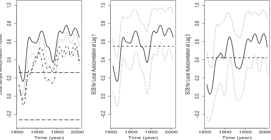
Figure 4. Left plot: local sample autocorrelation process ˆρk(t) in (8) withb=0.033 fork=1 (solid curve),k=2 (dotted curve),k=3
(dashed curve),k=4 (dot-dashed curve), along with the rule-of-thumb 95% simultaneous cutoff bands (SCBs; horizontal long-dashed lines) in (19) for testing for zero local autocorrelations. Middle plot and right plot: solid curve is the local sample autocorrelation process at lag 1 (middle plot) and lag 2 (right plot), the two dotted curves are the corresponding rule-of-thumb 95% SCB, and the horizontal long-dashed line, computed using (16), is the sample autocorrelation assuming stationarity.
90% and 95%, except that Model 3 withθ =1.0 has a slight undercoverage due to the strong dependence and nonlinearity. Furthermore, the bandwidth choiceb=1.5b∗ slightly outper-forms the other choicesb=b∗,2b∗. For the power study, as the model moves away from the null hypothesesH01 andH02, the power of the SCB-based test generally increases. Also, the pro-posed test forH01has better power thanH02. This phenomenon is due to the relatively larger magnitude of|ρ1(t)|than that of
|ρ2(t)|. In general, it is difficult to test the shape of a curve when the magnitude of the curve is too small. For example, for Model 2,ρ2(t)=[0.6{(1−θ)+θsin(2π t)}]2≤0.36, which explains the much lower power in testing forH2
0 thanH 1
0. For Model 3, the methods have comparable performance when we subtract either the nonparametrically estimated mean or the theoretical mean.
6. APPLICATIONS
Now we apply the methodology to the two examples in Sec-tion2.
6.1 Global Temperature Series in Section2.1
We study local autocorrelations for the global monthly tem-perature anomalies in Section 2.1. Denote by μ(t) the time-varying mean trend. Due to the clear time trend, we need to center the data first. Consider the local linear estimate ofμ(t) with Gaussian kernelK(·):
( ˆμ(t),μˆ′(t))=argmin (μ,μ′)
n
i=1
{Xi−μ−μ′(ti−t)}2K
ti
−t τ
.
(24)
To choose the bandwidthτ, we follow the discussions in Sec-tions 3.4and5 and letτ =1.5τ∗, whereτ∗ is the automatic bandwidth selected by the R function dpillassuming inde-pendence. The thick solid curve in Figure 1 is the estimated trend ˆμ(t). We then apply our methods to the centered data
˜
Xi=Xi−μˆ(i/n).
By the method in Section3.4, we use bandwidthb=0.033 in (8) for all k. The left plot of Figure 4 plots ˆρk(t) at lags k=1, . . . ,4. The four local sample autocorrelation processes exhibit similar but complicated time-varying patterns. Interest-ingly, there is a clear “V” shape during 1910–1960. To test for the null hypothesis of zero local autocorrelations, we plot 95% simultaneous cutoff bands in (19) as the two horizontal lines. Clearly, the null hypothesis is rejected, and the measurements are significantly positively correlated. To examine whether the local autocorrelations are indeed time-varying, in the middle and right plots ofFigure 4we plot ˆρ1(t) and ˆρ2(t) along with their 95% SCB, whereL=15≈2n4/15in (14). The horizontal lines, computed using (16), are not entirely contained within the SCB, thus we conclude that the local autocorrelations are indeed time-varying. Our findings suggest that the temperature series have an intrinsically complicated structure and should not be modeled by a mean trend plus a stationary noise as in the existing literature. A future research direction is to explore spe-cific time-varying coefficient models, such as the time-varying autoregressive models in Example 2.
6.2 S&P 500 Index Returns in Section2.2
By the discussion in Section2.2, we apply our local autocor-relations methodology to examine two important hypotheses: (i) the EMH that stock returns have zero autocorrelations; and
1995 2005
−0.4
−0.2
0.0
0.2
0.4
Time (year)
Local Sample A
utocorrelation f
or Retur
ns
1995 2005
−0.8
−0.6
−0.4
−0.2
0.0
0.2
0.4
Time (year)
Local Sample A
utocorrelation f
or Absolute Retur
ns
1995 2005
−0.2
0.0
0.2
0.4
0.6
0.8
1.0
Time (year)
Local Sample A
utocorrelation f
or Squared Retur
ns
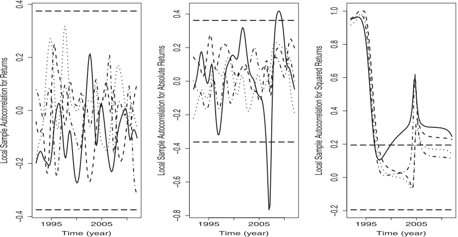
Figure 5. Left plot: local sample autocorrelation processes ˆρk(t) of logarithm returns fork=1 (solid curve),k=2 (dotted curve),k=3
(dashed curve),k=4 (dot-dashed curve), along with the rule-of-thumb 95% simultaneous cutoff bands (horizontal long-dashed lines) in (19) for testing for zero local autocorrelations. Middle plot and right plot: same as in the left plot but for centered absolute returns (middle plot) and squared returns (right plot).
(ii) the hypothesis that the absolute values or magnitudes of returns are correlated. Furthermore, numerous empirical stud-ies have shown that squared returns are positively correlated, a phenomenon that can be very well explained by the widely used ARCH/GARCH models. We shall also examine this phe-nomenon using our methods.
Figure 5 plots the local autocorrelations ˆρk(t) at lags k= 1, . . . ,4, along with the 95% simultaneous cutoff bands (hori-zontal long-dashed lines) in (19), for the returnsXi (left plot), the absolute returns|Xi|(middle plot), and squared returnsXi2 (right plot). When calculating ˆρk(t), we adopt the following rule: (i) do not center the returns; (ii) use local linear regression to center |Xi|, that is,|Xi| −μˆ(ti); and (iii) subtract the sample mean squared returns to centerX2
i, that is,X
2
i −n−
1n
i=1X 2
i. The rationale is to avoid local linear regression (which always introduces estimation errors) when the mean trend is weak rel-ative to the strength of autocorrelations. See Section 3.2for detailed explanations.
FromFigure 5, we make the following observations: First, in the left plot, since all the curves ˆρ1(t), . . . ,ρˆ4(t) are contained within the cutoff bands, we have no evidence to reject the null hypothesis of zero local autocorrelations. Thus, we conclude that the returns are uncorrelated, which confirms the EMH that it should be impossible to predict stock returns.
Second, in the middle plot, since ˆρ1(t) is not entirely con-tained within the bands, we reject the null hypothesis of zero lo-cal autocorrelations at the 5% significance level. Thus, although the returns are uncorrelated, the absolute returns are signifi-cantly correlated at lagk=1. Our conclusion is consistent with those in Fama (1970) and Ding, Granger, and Engle (1993). It is worth pointing out that, the absolute values of returns are impor-tant in risk management. For example, a risk-aversion investor
may want to stay on the sidelines when he/she expects large magnitudes of returns, equally likely to be positive or negative. Interestingly, comparing the left plot ofFigure 2and the middle plot ofFigure 5, we see that the peaks and bottoms of the stock market correspond to the bottoms and peaks of the local auto-correlation process ˆρ1(t) of the absolute returns. For example, the stock market peaked in 2007 when the local autocorrelation bottomed; the subsequent financial crisis during 2008 and early 2009 corresponds to a dramatic increase in ˆρ1(t) with a peak at approximately the time when the market bottomed.
Third, the right plot suggests significant and mostly positive local autocorrelations for the squared returns, which is consis-tent with the ARCH/GARCH modeling in existing literature. A future research direction is to investigate specific time-varying coefficient ARCH/GARCH models (see Example 4) with non-parametrically estimated coefficients and data-driven order se-lection.
APPENDIX: PROOFS
Theorem A.1. Recall ti and ξi in (1). Define ηi=h(ti, ξi) for a
transformationh(·,·) such thatE(ηi)=0. LetHn(t)=
n
i=1K{(ti−
t)/b}ηi. Supposeh∈SLC(2)-GMC(4) (see Assumption 1),K(·)
satis-fies Assumption 2(i),b→0 andnb2/(logn)8
→ ∞. Further assume
2(t) :
=var{h(t, ξ0)} +2
∞
r=1cov{h(t, ξ0), h(t, ξr)}>0 for allt∈
[0,1]. Then
1. [Asymptotic normality] For each fixed t∈(0,1), (nb)−1/2H
n(t)/(t)⇒N(0, ϕK).
2. [Maximum deviation] Let CK be defined in Theorem 2. For all
ditionh∈SLC(2)-GMC(4) (recall that this condition imposes a finite fourth moment; see Assumption 1), there exist iid standard normal variablesZ1, . . . , Znsuch that
By (A.1) and the summation by parts again,
Hn(t)=
it suffices to establish the corresponding results for the Gaussian pro-cessn
i=1Ki(ti)Zi.
(i) It easily follows sinceZ1, . . . , Znare iid N(0,1). (ii) It follows
from the maximum deviation of the Gaussian processn
i=1Ki(ti)Zi
(Lemma 2 in Wu and Zhao2007).
Proof of Proposition 2. By Isserlis (1918), for any
nor-mal vector (Z1, Z2, Z3, Z4) with zero mean, E(Z1Z2Z3Z4)= E(Z1Z2)E(Z3Z4)+E(Z1Z3)E(Z2Z4)+E(Z1Z4)E(Z2Z3). Using this
identity and after some careful calculations, we can show the result.
Proof of Theorems 1 and 2. RecallE[g(t, ξ0)]=0. Forγk(t) in (4),
By Assumption 1(i) and the Schwarz inequality,
E|g(ti, ξi)[g(ti+k, ξi+k)−g(ti, ξi+k)]| ≤ g(ti, ξi)2× g(ti+k, ξi+k)−
from the asymptotic normality and maximum deviation ofWn(t) via
Theorem A.1.
ACKNOWLEDGMENTS
The authors are grateful to an associate editor and a referee for their constructive comments. Zhao’s research was supported by an NSF grant DMS-1309213 and an NIDA grant P50-DA10075-15. The content is solely the responsibility of the authors and does not necessarily represent the official views of the NIDA or the NIH.
[Received July 2013. Revised July 2014.]
References
Adak, S. (1998), “Time-Dependent Spectral Analysis of Nonstationary Time Series,”Journal of the American Statistical Association, 93, 1488–1501. [296]
Andel, J., Netuka, I., and Svara, K. (1984), “On Threshold Autoregressive Processes,”Kybernetika, 20, 89–106. [298]
Bickel, P. J., and Rosenblatt, M. (1973), “On Some Global Measures of the Deviations of Density Function Estimates,”The Annals of Statistics, 1, 1071–1095. [296]
Dahlhaus, R. (1997), “Fitting Time Series Models to Nonstationary Processes,” The Annals of Statistics, 25, 1–37. [296,298]
——— (2012), “Locally Stationary Processes,” in Handbook of Statistics, Time Series Analysis: Methods and Applications(Vol. 30), eds. T. Subba Rao, S. Subba Rao, and C. R. Rao, Amsterdam: North Holland, pp. 351– 413. [296]
Dahlhaus, R., and Subba Rao, S. (2006), “Statistical Inference for Time-Varying ARCH Processes,”The Annals of Statistics, 34, 1075–1114. [296,299] Davis, R. A., Lee, T., and Rodriguez-Yam, G. (2006), “Structural Break
Esti-mation for Nonstationary Time Series Models,”Journal of the American Statistical Association, 101, 223–239. [296]
Ding, Z., Granger, C. W. J., and Engle, R. F. (1993), “A Long Memory Property of Stock Market Returns and a New Model,”Journal of Empirical Finance, 1, 83–106. [297,304]
Eubank, R. L., and Speckman, P. L. (1993), “Confidence Bands in Nonpara-metric Regression,”Journal of the American Statistical Association, 88, 1287–1301. [296]
Fama, E. (1970), “Efficient Capital Markets: A Review of Theory and Empirical Work,”Journal of Finance, 25, 383–417. [297,304]
Fan, J., and Zhang, W. (2000), “Simultaneous Confidence Bands and Hypothesis Testing in Varying-coefficient Models,”Scandinavian Journal of Statistics, 27, 715–731. [296]
Isserlis, L. (1918), “On a Formula for the Product-Moment Coefficient of Any Order of a Normal Frequency Distribution in Any Number of Variables,” Biometrika, 12, 134–139. [305]
Lahiri, S. N. (2003),Resampling Methods for Dependent Data, New York: Springer-Verlag. [301]
Mallat, S., Papanicolaou, G., and Zhang, Z. (1998), “Adaptive Covariance Es-timation of Locally Stationary Processes,”Annals of Statistics, 26, 1–47. [296]
Nason, G. P., Von Sachs, R., and Kroisandt, G. (2000), “Wavelet Processes and Adaptive Estimation of the Evolutionary Wavelet Spectrum,”Journal of the Royal Statistical Society, Series B, 62, 271–292. [296,301]
Ombao, H., Raz, J., Von Sachs, R., and Malow, B. A. (2001), “Automatic Statistical Analysis of Bivariate Nonstationary Time Series,”Journal of the American Statistical Association, 96, 543–560. [296]
Ombao, H., Von Sachs, R., and Guo, W. (2005), “SLEX Analysis of Multivariate Nonstationary Time Series,”Journal of the American Statistical Association, 100, 519–531. [296]
Priestley, M. B. (1965), “Evolutionary Spectra and Non-Stationary Processes,” Journal of the Royal Statistical Society,Series B, 27, 204–237. [296] Priestley, M. B., and Chao, M. T. (1972), “Non-parametric Function Fitting,”
Journal of the Royal Statistical Society, Series B, 34, 385–392. [300] Ruppert, D., Sheather, S. J., and Wand, M. P. (1995), “An Effective Bandwidth
Selector for Local Least Squares Regression,”Journal of the American Statistical Association, 90, 1257–1270. [300]
Rust, B. W. (2003), “Signal From Noise in Global Warming,”Computing Sci-ence and Statistics, 35, 263–277. [297]
Subba Rao, T. (1970), “The Fitting of Nonstationary Time Series Models With Time-dependent Parameters,”Journal of the Royal Statistical Society, Series B, 32, 312–322. [296,298]
Van Bellegem, S., and Von Sachs, R. (2008), “Locally Adaptive Estima-tion of EvoluEstima-tionary Wavelet Spectra,”The Annals of Statistics, 36, 1879– 1924. [296,301]
Woodward, W. A., and Gray, H. L. (1993), “Global Warming and the Problem of Testing for Trend in Time-series Data,”Journal of Climate, 6, 953–962. [297]
Wu, W. B., Woodroofe, M., and Mentz, G. (2001), “Isotonic Regression: Another Look at the Change Point Problem,” Biometrika, 88, 793– 804. [297]
Wu, W. B., and Xiao, H. (2012), “Covariance Matrix Estimation in Time Series,” inHandbook of Statistics(Vol. 30). [296]
Wu, W. B., and Zhao, Z. (2007), “Inference of Trends in Time Series,”Journal of the Royal Statistical Society, Series B, 69, 391–410. [296,297,305] ——— (2011), “Gaussian Approximations for Non-Stationary Multiple Time
Series,”Statistica Sinica, 21, 1397–1413. [296,298,300,305]