www.elsevier.nl / locate / econbase
Fair-negotiation procedures
* Matthias G. Raith
Institute of Mathematical Economics, University of Bielefeld, P.O. Box 100131, D-33501 Bielefeld, Germany
Received 31 July 1998; received in revised form 31 March 1999; accepted 31 March 1999
Abstract
In this paper we reformulate three fair-division algorithms as practical, cooperative negotiation procedures that can be applied to a more general class of multiple-issue negotiations. The procedures consist of two simple and intuitive steps: the first step ensures an efficient outcome, and the second step establishes ‘fairness’ through a redistribution of gains. For all procedures we also compare the outcomes of ‘issue-by-issue’ negotiations and ‘package deals.’ 2000 Elsevier Science B.V. All rights reserved.
Keywords: Bargaining; Fair division; Multi-issue negotiations
1. Introduction
In contrast to ‘normative’ mathematical models of bargaining or ‘descriptive’ analyses of actual negotiations, negotiation analysis is a practically oriented field of research that can be characterized as ‘prescriptive’, meaning that the objective is to give procedural
1
advice on how negotiators can reach a mutually beneficial outcome. However, despite its theoretical orientation, one cannot claim that negotiation analysis is firmly rooted in
2 bargaining or, more generally, game theory.
The practical deficit of ‘cooperative’ game theory, on the one hand, is that the characterization of the game does not include the ‘plan of play’. Axiomatic solution concepts focus on the desirable properties of bargaining solutions, but they do not
*Tel.: 149-521-106-5646; fax:149-521-106-2997. E-mail address: [email protected] (M.G. Raith)
1
For an overview of the wide range of topics belonging to negotiation analysis, see the book edited by Young (1991).
2
Sebenius (1992), for example, even takes a strong stand for ‘‘a de-emphasis on game-theoretic solution concepts.’’
specify the process that leads to them. This has spurred the development of ‘non-cooperative’ or strategic bargaining games, on the other hand, as an attempt to model bargaining procedures that lead to or approximate axiomatic solutions. The latter approach is debatable, though, because the characterization of a specific bargaining procedure makes it difficult to derive general implications. Moreover, the strictly non-cooperative behavior of the players must be viewed critically: even when parties have strongly conflicting interests, it would be a mistake to automatically infer that the negotiators themselves behave non-cooperatively. Indeed, many descriptions of profes-3 sional political or business negotiations seem to indicate a more cooperative attitude.
According to Brams and Taylor (1996), bargaining theories have proved inapplicable to the settlement of real-life disputes because of their divorce from theories of fair division. They show that, by viewing negotiation problems as problems of fair division, one can apply intuitive procedures to a variety of complex conflicts. The important feature of this approach, however, is not its view of negotiation as a fair-division problem. The relevant aspect is the applicability of fair-division procedures to conflicts
4
in general. A basic requirement is that they are simple enough to follow without specific training and plausible enough to argue.
In this paper, instead of viewing negotiation problems as fair-division problems, we reformulate fair-division procedures as cooperative negotiation procedures, in order to apply them to general multiple-issue negotiations. A fair-division problem is a special type of negotiation problem, where the negotiated issues are the items to be divided. To force a multiple-issue negotiation problem into this tighter corset thus requires additional simplifying assumptions. As a consequence, a fair-division procedure generally does not acknowledge the full problem.
We focus here on bilateral problems where items or issues are valued by both parties in some common standard of value, e.g. a unit of money. If items can be valued in terms of money, then a fair-division procedure based on a bidding procedure seems intuitive. This concept was developed by Knaster (1946) and Steinhaus (1948). We refer to it here
5
as the ‘Knaster procedure.’ With this simple method, items are assigned to the players who value them most, and ‘fairness’ is established through monetary transfers. The resulting division is ‘efficient’ and for two parties also ‘envy-free’, meaning that neither player would want to trade shares with the other. However, due to its rigid transfer mechanism, the outcome is not ‘equitable,’ meaning that players do not enjoy equal
6 relative gains.
Brams and Taylor (1996) see a major advantage in their procedure ‘Adjusted Winner,’ which acknowledges this additional, and apparently relevant, criterion of fairness. The algorithm is closely related to the Knaster procedure, but the transfer
3
In his recent ‘lectures’, Raiffa (1996) devotes most of the analysis to situations where negotiators are engaged in what he refers to as ‘‘full open truthful exchange’’.
4
Brams and Taylor (1999) present a variety of qualitatively different examples that illustrate this point.
5
While Raiffa (1982) refers to the ‘Steinhaus procedure,’ Brams and Taylor (1996) argue that the procedure should, in fact, be attributed to Knaster (1946) who formulated it first.
6
mechanism is specifically designed to establish equitability. In addition, the fair division does not require money, since the transfer is achieved by shifting items. This feature is extremely useful for fair-division problems, where items cannot be valued in terms of money, or when parties do not have access to extra money for compensation.
However, when side payments are possible, Adjusted Winner may be too restrictive. We, therefore, take the ‘best’ of both procedures by combining the efficient side payments of the Knaster procedure with the equitability condition of Adjusted Winner. We acknowledge its individual components by naming this new method of fair division ‘Adjusted Knaster.’ By imposing an equitable monetary transfer, Adjusted Knaster implements an equitable outcome that is always as least as good as that of Adjusted Winner.
We generalize the fair-division procedures in order to apply them to multiple-issue, multiple-option negotiations. We formulate the algorithms as intuitive two-step pro-cedures. The first step implements an efficient outcome, and it is the same for all three procedures. They differ in the second step, though, which establishes ‘fairness’ through a redistribution of gains.
We show that the adjustment mechanisms have different procedural implications, when they are used in ‘issue-by-issue’ negotiations. This form of negotiation has a high practical relevance, since it reduces the complexity and allows negotiators to follow an agenda. Although axiomatic solution concepts do not tell us how to implement a cooperative solution, we find them to be useful for designing cooperative implementa-tion procedures that meet practical requirements.
Our approach in this paper is complementary to that of Raiffa (1996), who shows how the use of computer spread-sheet analysis can provide strong negotiation-analytic support. The important difference of our procedural view here is that it is focused on argumentative support and does not require computer assistance.
In order to illustrate the applicability of the three ‘fair-negotiation’ procedures, we choose an existing problem taken from Gupta (1989). In this marketing negotiation between a manufacturer of multiple products and a large retailer, players negotiate over six different marketing plans for each of six different products. Thus, the problem features enough complexity in order to assess the potential of the procedures.
The paper is structured as follows. In Section 2 we analyze a simple fair-division problem and compare the solutions of Adjusted Winner and the Knaster procedure. As an alternative we introduce ‘Adjusted Knaster.’ In Section 3 we describe a multi-issue negotiation problem, where both players value options by the same standard of value, viz. money. In Section 4 we characterize the three fair-negotiation procedures, and in Section 5 we analyze their performance in issue-by-issue negotiations. Practical conclusions of our analysis are given in Section 6.
2. Fair-division procedures
Table 1
freak, values both highly at 100 Dollars. Player R sees them mainly as souvenirs, and values the photo collection at 30 Dollars and the painting at 10 Dollars. Both players’ subjective valuations of the estate are given in Table 1. The question is: What is a fair division?
Player M is indifferent between both items, but player R clearly prefers item 1. If one item is given to each player, then R will presumably ask for item 1, leaving item 2 for player M. In percentage terms, M receives 50% of the estate, while R can reap 75% for
7
herself. There is no redistribution of items that makes both players better off, and no player alone will want to trade items either. The allocation is thus ‘efficient’ and ‘envy free’.
The question arises, though, whether the distribution procedure should take into account that player M values the photo collection (item 1) more than three times as much as player R who, nevertheless, gets it. Indeed, if the two players were to bid for these items in an auction, both would go to player M.
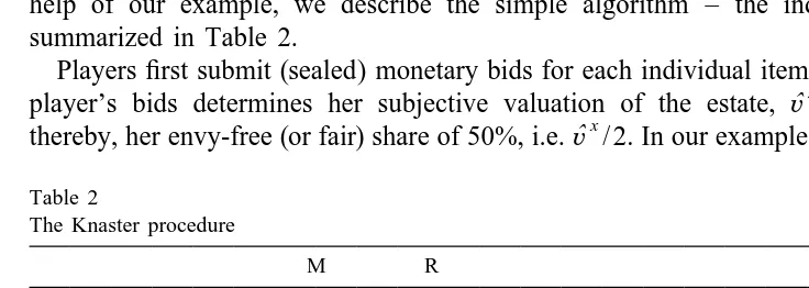
The idea of a fair-division procedure based on an auction was developed by Knaster (1946) and Steinhaus (1948). We refer to it here as the ‘Knaster procedure.’ With the help of our example, we describe the simple algorithm – the individual steps are summarized in Table 2.
Players first submit (sealed) monetary bids for each individual item. The sum of each
x
ˆ
player’s bids determines her subjective valuation of the estate, v (x5M,R), and,
x
ˆ
thereby, her envy-free (or fair) share of 50%, i.e.v / 2. In our example, player M expects
Table 2
The Knaster procedure
M R
1. Photo collection 100] 30 2. Oil painting 100] 10
to receive a share of the estate worth at least 100, while player R would surely complain about a share worth less than 20.
Each item is assigned to the highest bidder. If players bid the same amount for an item, then a referee decides. Summing over all assigned items then yields each player’s
x
received value,v (x5M,R), and, thus, her excess over her fair share. In our example,
T
player M receives both goods which gives her twice as much as her fair share. In contrast, player R receives nothing, which is why her excess is 220.
The Knaster procedure splits the total excess E, in our example 80, evenly among the 8
players. Since player M should receive a share of the excess worth only 40, she must pay 100240560 to R. Player R is compensated for her loss of 20 and, in addition, receives her half of the excess, giving her a total of 20140560. Hence, all transfer
x M R x x
ˆ
payments t cancel out, i.e. t 1t 50. Players’ total values are then v 5(v 1E ) / 2
(x5M,R).
By introducing side payments in terms of the standard of value, the Knaster procedure introduces a form of compensation that is more efficient than the redistribution of goods. In our example, M’s valuation of item 1 is three times as high as R’s in terms of money. Or, the other way around: R’s valuation of money is three times as high as M’s in terms of item 1. Consequently, M is better off compensating R with money rather than with item 1.
The outcome of the Knaster procedure is that M receives a total value of 140, while R gets 60. In percentage terms, M receives 70% of the estate and R even gets 150%. Compared with the previous envy-free distribution, both players now have significantly more. Nevertheless, player M may feel unsatisfied, because R got much more of what she wanted. Although the division is ‘efficient’ and ‘envy-free,’ it is not ‘equitable.’ In fact, R’s share is higher than her valuation of the complete estate, which appears somewhat absurd.
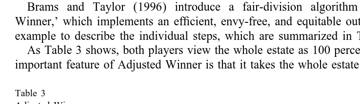
Brams and Taylor (1996) introduce a fair-division algorithm called ‘Adjusted Winner,’ which implements an efficient, envy-free, and equitable outcome. We use our example to describe the individual steps, which are summarized in Table 3.
As Table 3 shows, both players view the whole estate as 100 percent of the ‘pie.’ An important feature of Adjusted Winner is that it takes the whole estate as the standard of
Table 3 Adjusted Winner
M R
1. Photo collection 50 75] 2. Oil painting 50] 25
value, rather than some monetary unit. This makes the algorithm particularly interesting for problems of fair division, where the items cannot all be valued in terms of money. In that case, it may be much simpler for players to allocate 100 percentage points among the items to be divided.
9 In a first step, Adjusted Winner assigns each item to the player who values it most. Item 1 now goes to player R and item 2 to player M. This allocation determines that R is the ‘temporary winner’ and M the ‘temporary loser.’ The main aspect of this procedure
10
is that the outcome of step 1 is guaranteed to be efficient: By giving each item to the player who values it higher, the sum of both players’ utilities is maximized for each issue. Therefore, the sum of their utilities is also maximized over all issues together. Hence, the outcome is efficient, since there is no outcome that can give both players a higher utility.
In a second step, Adjusted Winner redistributes items from the temporary winner to the temporary loser at the lowest cost–gain ratio in order to maintain efficiency. In our simple example, only item 1 can be shifted from R to M. Since this would give M 100% and leave R with nothing, equitability requires a division of item 1. If M receives 20% of the photo collection and R 80%, then each player, in her view, will end up with 60% of the whole estate (cf. Table 3).
Despite the equitability and the efficiency of the outcome, one may question, though, whether Adjusted Winner is the most plausible procedure for this fair-division problem. Note that players are both worse off than with the Knaster procedure. The reason, of course, is that equitability requires players to divide item 1 instead of money.
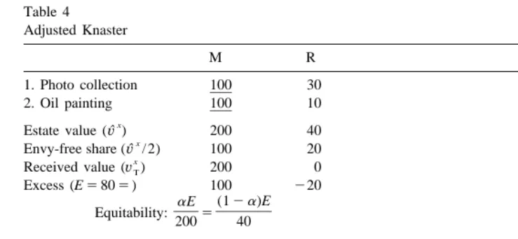
Intuitively, one can expect to obtain a better outcome by marrying the efficient adjustment method of the Knaster procedure with the equitability condition of Adjusted Winner. By doing this, we construct a method of fair division which we call ‘Adjusted Knaster.’ As Table 4 shows, the procedure is just as simple as its ‘parents.’
Adjusted Knaster first follows the Knaster procedure by giving both items to player M, so that the total excess is again equal to E5100220580. Now, however, the excess is not split evenly. Since both players value the estate differently, their valuation of the monetary excess in terms of the estate is not the same. Therefore, in the second step, Adjusted Knaster equalizes the players’ shares of the excess in relation to their valuation of the estate. Instead of 1 / 2, player M now receives a 55 / 6 of the excess, which she values at 1 / 3 of the estate, the same as player R values her share of
R M
12a 51 / 6 of the excess. As a consequence, the required transfer to R, t 5 2t ,
reduces to 33.33. Since this leaves both players with 83.33% of the estate, the outcome of Adjusted Knaster is equitable. We formalize this result in the following theorem.
Theorem 1. Assume that the‘excess’ value, defined as the difference between the total
value of received items and the sum of the envy-free (50%) shares, is distributed
through monetary transfers. If players receive an equitable share of the excess, then they
will also receive an equitable share of the estate. Moreover, their share of the total
value of received items is equal to their share of the excess.
9
If items are valued equally by both players, then a referee can decide.
10
Table 4 Adjusted Knaster
M R
1. Photo collection 100] 30
2. Oil painting 100] 10
Proof. Denote players’ valuation of the estate by v and v , respectively. With
a[[0,1] denoting player M’s share of the excess E, equitability implies that
aE (12a)E
equation, one obtains the equivalent condition
M R
The denominators on both sides of this equation are equal to the values of the final
M R
outcomes, v andv , such that
M R
v v
]M5]R,
ˆ ˆ
v v
which proves the first part of the theorem. In order to show the second part, note that the final outcomes are simply a redistribution of the total value of received items. With
The second part of the theorem shows that Adjusted Knaster is even simpler than Table 4 suggests. In order to determine the transfer payment, one only needs players’ valuation of the estate and the total value of received items. There is no need to calculate the excess.
Compared with the outcome of Adjusted Winner, the improvement through Adjusted Knaster is substantial. Two critical aspects need to be mentioned, though. First, Adjusted Knaster requires a common standard of value (e.g., money) for each item. This restricts the procedure’s applicability, since there are many fair-division problems where a valuation of all items in terms of money is not possible or may even be considered as immoral. Second, a side payment requires money, which the paying party simply may not have. Brams and Taylor (1996) emphasize that Adjusted Winner is immune to both of these weaknesses, since it is a pure point-allocation procedure.
On the other hand, Adjusted Winner generally requires that one of the items is divided. Fortunately, the division involves at most one item, but it is not certain that this particular item is divisible and how players value fractions of it. Indeed, dividing an item can be just as problematic as assigning to it a monetary value. Adjusted Knaster requires no division of goods whatsoever, since it establishes equitability through a monetary transfer. Hence, Adjusted Knaster may be seen as the natural extension of Adjusted Winner, when side payments are possible.
Problems of fair division concerning multiple items are special cases of multiple-issue negotiations. In order to see this, we interpret our example as a negotiation problem over two issues (i.e. the items), where for each issue there are two discrete options – option 1: M gets the item and R gets nothing; and option 2: R gets the item and M gets nothing.
2
With two issues, there are 2 54 discrete outcomes. If the items are divisible – which Adjusted Winner requires – one can also consider convex combinations of options. Formally, we assume that players’ preferences are characterized by utility functions
x 2 x
v : [0,1] →R(x5M,R), where v is assumed to be linear on the pair of divisions. In
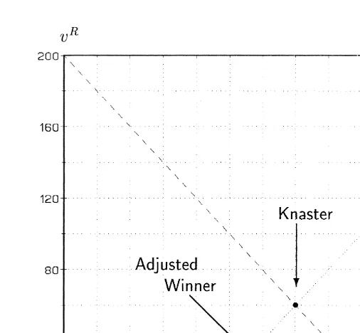
particular, this implies that players’ utilities are additively separable across issues. Fig. 1 shows the four discrete outcomes, denoted by ‘+’. The solid line indicates the efficient boundary of the bargaining set.
Fig. 1 also shows the outcomes of the three fair-division procedures. The outcomes of the Knaster procedure and Adjusted Knaster are located on the negatively sloped 458 line passing through the allocation (200,0), since both involve monetary transfers. The Knaster outcome is at the intersection with the positively sloped 458line passing through the 50% allocation, denoted by ‘1’ at (100,20). Adjusted Knaster has its outcome at the intersection with the equitability line, which indicates equal percentage gains for both players; its slope is given by the ratio of players’ valuations of the estate. Adjusted Winner implements an outcome on the Pareto frontier of the bargaining set at the intersection with the equitability line. Fig. 1 clearly illustrates how Adjusted Knaster extends Adjusted Winner. Under Adjusted Knaster, players always do at least as well as under Adjusted Winner.
Fig. 1. Outcomes of fair-division procedures.
scale invariance. Since the point allocation is a normalization method, it rescales payoffs at a constant factor. This affects the individual steps of Adjusted Winner, but not its final outcome. With the valuations given in Table 1, the first step gives both items to player M, analogous to the other two procedures. The second step then transfers items from M to R at the most efficient rate. The equitable allocation involves the same division of item 1.
3. A multiple-issue multiple-option negotiation
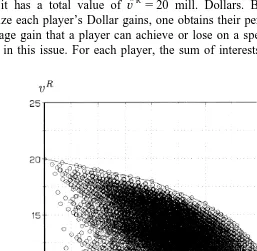
Consider now a negotiation between a manufacturer (M) and a retailer (R) over six different marketing plans (A–F) for each of six different products (1–6). We borrow the example of Gupta (1989), which features the structure and complexity of marketing negotiations that have been studied in the literature. Table 5 shows both negotiators’ gains for each of the marketing plans in units of one mill. Dollars.
The six different products are the issues of this negotiation. An option is a marketing plan A–F for each of the products 1–6. An agreement consists of one plan for each
6
product. If no option is divided, then there are 6 546,656 possible agreements to this
M R
negotiation. Fig. 2 shows players’ total gains,v andv , for each discrete outcome. As
the picture shows, the complexity of this negotiation far exceeds that of a fair-division 6
Table 5
Gains of players M and R from plansA–Ffor products 1–6
Issues Options Max
A B C D E F
1 M 0.00 1.65 3.00 3.66 5.00 6.00 6.00
R 2.00 1.65 1.40 1.22 1.00 0.00 2.00
2 M 0.00 0.72 1.20 1.50 1.70 2.00 2.00
R 2.00 1.50 1.20 1.00 0.60 0.00 2.00
3 M 2.00 1.70 1.50 1.20 0.72 0.00 2.00
R 0.00 0.60 1.00 1.20 1.50 2.00 2.00
4 M 0.00 1.00 1.25 1.50 1.80 2.00 2.00
R 8.00 6.67 5.00 4.00 1.72 0.00 8.00
5 M 6.00 5.00 3.66 3.00 1.65 0.00 6.00
R 0.00 1.00 1.22 1.40 1.65 2.00 2.00
6 M 0.00 1.40 2.80 3.75 5.00 6.00 6.00
R 4.00 3.40 2.80 2.50 2.00 0.00 4.00
M
ˆ
over all six issues. For player M, the complete pie is worthv 524 mill. Dollars, while
R
ˆ
for R, it has a total value of v 520 mill. Dollars. By using these two values to
normalize each player’s Dollar gains, one obtains their percentage gains. The maximum percentage gain that a player can achieve or lose on a specific issue can be seen as her interest in this issue. For each player, the sum of interests is equal to 100 percent. The
two characterizations of utilities are the same as in the preceding section, but since it is more natural to assume that a negotiation between a manufacturer and a retailer is conducted in terms of Dollars, we maintain this characterization in the following analysis.
For a direct application of the fair-division procedures of the preceding section, we need to assume that players view issues as items that can be divided between them. With linear, additively separable utility functions, players’ preferences are characterized by their interests in complete issues, i.e. by the values of their best options. In Table 5 this is captured in the right-hand column.
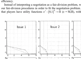
Applying a fair-division procedure to the negotiation problem of Table 5, however, will generally lead to an inefficient outcome. This is because the linearization of preferences regards only convex combinations between the best and the worst options and, thereby, blends out efficient intermediate agreements. This is shown in Fig. 3, where we have plotted players’ gains for each of the six issues. By choosing the same scale for each graphic, one can see the relative importance of the individual issues for both players. The six hollow points in each panel denote the individual options. The dashed lines illustrate how the assumption of linear preferences leads to a loss of efficiency.
Instead of interpreting a negotiation as a fair-division problem, we wish to reformulate our fair-division procedures in order to fit the negotiation problem. We therefore assume
x 6 x x x
that players have utility functions v : [0,1] →R (x5M,R), with v ;v 1v 1 ? ? ?
1 2
x x
1v , where the subutility functions, v , i51, . . . ,6, are now assumed to be piecewise
6 i
linear and concave. The solid lines in the six panels of Fig. 3 indicate the efficient boundaries for the individual issues. Note that not all options are efficient if convex combinations are possible. The solid line in Fig. 2 shows the efficient boundary of the negotiation problem over all six issues together. In order to adapt the fair-division procedures of Section 2 to this more general negotiation problem, we do not change their individual steps, but only phrase them more generally.
4. Fair-negotiation procedures
An important aspect to be learned from the fair-division procedures is that the issue-option characterization in Table 5 contains more structural information than the joint payoffs of package agreements shown in Fig. 2. This additional information allows us to construct procedures that do not require computer support.
In payoff space, all three fair-division procedures first assign the individual issues to the player who values them most. The reason why this induces an efficient outcome is because, with linear preferences, the sum of both players’ payoffs is maximized. With this goal in mind, we are able to formulate the first step of our fair-negotiation procedures.
Step 1. For each issue i choose the ‘temporary options’ iT that maximize the sum of
M R
players’ gains, i.e. iT[argmax hv 1v j. If more than one option satisfies this
T iT iT
criterion, then let a referee decide which option to choose from this set. All temporary
options, together, constitute the ‘temporary agreement.’ The sum of each player’s
x x
temporary gains, v 5ov (x5M,R), determines the ‘temporary winner’ W and the
T i iT
‘temporary loser’ L through the condition
W L
We illustrate step 1 with the help of our example. For issue 1, the sum of payoffs is maximized with options E and F, which both yield a total gain of 6. Either can be chosen as the temporary option. Presumably, players would select the less extreme optionE. For issue 2, the temporary option isD, for issue 3, it is optionC, and for issue 4, the joint maximum is with optionA. Issue 5 offers a choice again between optionsA and B, where we assume that players would pick B. For issue 6, optionE maximizes joint gains. The ‘temporary agreement’ is then given by the 6-tuple of options
M R
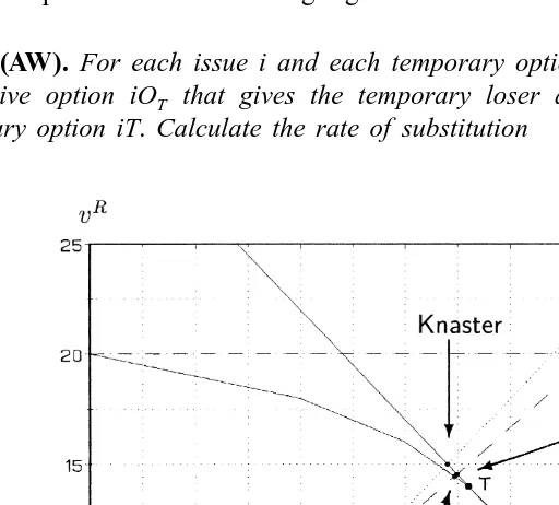
[EDCABE], which yields total payoffs ofv 518 andv 514. In Fig. 4, the temporary
T T
outcome is denoted by T.
Since step 1 maximizes the sum of payoffs for each individual issue, it also maximizes the sum of payoffs over all issues together. Hence, the outcome is efficient, because there is no agreement which yields a higher gain for both players. The outcome of step 1 matches that of the utilitarian solution characterized by Myerson (1981).
458 line with the efficiency frontier. As Fig. 4 shows, the temporary outcome is not unique. This is because step 1 offers a choice of alternatives for issues 1 and 5. At point T, players outcomes yield
M R
v 18 14 v
T T
]M5]2450.75.0.705]205]R.
ˆ ˆ
v v
According to the condition of step 1 above, player M is the temporary winner and player R the temporary loser. For all three of our fair-negotiation procedures, we take outcome T as the starting point of step 2. The final outcomes of the three algorithms are illustrated in Fig. 4.
4.1. Adjusted Winner
Adjusted Winner redistributes gains by switching options with the aim of achieving equitability. Since step 1 already has an efficient outcome, the adjustment rule must be designed in order to keep players on the efficiency frontier. We describe the complete adjustment process in the following algorithm.
Step 2 (AW). For each issue i and each temporary option iT, consider each efficient
alternative option iOT that gives the temporary loser a higher gain than with the temporary option iT. Calculate the rate of substitution
W W
Select the alternative options iOT that yield the lowest cost –gain ratio, i.e. iOT [ argmin RSO i :TOT. If more than one option satisfies this criterion, then let a referee choose
*
from this set. Now determine the issues i with the lowest cost –gain ratio, i.e. *
i [argmin RSi i :TO*T. If there is no unique issue, then let a referee decide. Calculate
W L
*
players’ overall utilities v * and v * by replacing only option i T with its efficient
OT OT
then make i OT the new temporary option of issue i and repeat step2. Else, calculate * * *
the convex combination of options i T and i OT that equalizes the relative gains between the winner W and loser L. x
In order for the adjustment process to maintain efficiency, the transfer from the temporary winner to the temporary loser must be achieved at a minimum cost–gain ratio. With a piecewise linear Pareto frontier connecting discrete agreements, a movement along the efficient boundary requires switching only one option at a time. In order to find the efficient option switch, one must only find the best alternative within
11 each issue, and then select the best alternative among all issues.
For issue 1 in our example, the temporary option isE. Among the alternativesD,C, B, and A, options C and A both allow an efficient shift from player M to R, with RS1:EC5RS1:E A55. For issue 2, there are also two efficient alternatives, since RS2:DC5RS2:DA51.5. The same is true for issue 3, where RS3:CD5RS3:CF51.5. Issue 4 offers no possibility of substitution, since player M is at her minimum here. Issue 5 has options D and F as the efficient alternatives to B, with RS5:BD5RS5:BF55. Finally, for issue 6 the efficient alternatives to option E are D and A, with RS6:ED5 RS6:E A52.5. The cheapest possibility of substitution from player M to R is thus given by issues 2 and 3. If players select issue 2 and begin with the smaller step of shifting to option 2C, the new agreement yields
M R
According to the algorithm of Adjusted Winner, they must repeat step 2. They now have the choice of taking a larger step from option 2Cto 2Aor a smaller step from 3Cto 3D, since both have the same substitution rates. The latter brings them to the agreement [ECDABE]. With
11
M R
equitability is almost achieved. Indeed, if players now shift from 3Dto 3F, the outcome implies
Equitability thus requires a convex combination of options 3D and 3F. Denoting the relative weight of option 3D by a, the equitability condition becomes
M R
implying a value of a 50.94. The equitable agreement [EC(0.94D10.05F)ABE]
] ]
M R
yields the payoffsv 517.33 andv 514.44, giving each player a percentage increase
] of 72.22%.
It is important to note that, at each ‘referee decision’ of step 2, players could take an alternative route leading to a different agreement, but with the same payoff. For example, players could remain at option 2Dand concentrate their adjustment process on issue 3. The final agreement could then be of the form [ED(bD1(12b)F)ABE], with
]
b 50.694. Hence, each referee decision gives negotiators more room to maneuver, without increasing the conflict, since their payoffs are unaffected.
Finally, any efficient agreement requires the convex combination of at most two options of only one single issue. This aspect is of great practical importance, because negotiators, attempting to reduce complexity, often follow the procedure of seeking a compromise on each individual issue. We deal with this aspect in Section 5.
4.2. Knaster
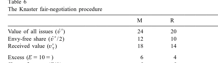
If negotiators value options with the same standard of value (in our example money), they might also have the possibility of redistributing gains through transfers of this common standard. In Section 2 we have seen that the Knaster fair-division procedure includes a simple transfer mechanism that leaves both negotiators with the same monetary excess over their envy-free share of 50%. The application of this procedure to a more general negotiation problem is straightforward. As for Adjusted Winner, we formulate the adjustment process in the form of an algorithm. For our example, the individual steps of the procedure are given in Table 6.
Step 2 (KN). Make the temporary agreement the final agreement. Determine each
x
player’s ‘transfer’ t as the difference between her share (50%) of the total excess and
her individual excess or, equivalently
Table 6
The simplicity of the Knaster procedure is remarkable: Players M and R agree on the combination of options [EDCABE], and player M pays R a compensation of 1 mill. Dollars. Moreover, the sum of players’ total payoffs (17115532) is higher than with
] ] ]
Adjusted Winner (17.3114.4531.7). In Fig. 4 the outcome of Adjusted Winner is below the negatively sloped 458 line. As before, the only disturbing feature of the Knaster procedure is that the outcome is generally not equitable.
4.3. Adjusted Knaster
In order to obtain an equitable outcome, we can formulate the algorithm of Adjusted Knaster analogously to the Knaster procedure. The only difference is that players receive an equitable rather than an equal share of the excess. However, the procedure becomes even simpler if we make use of Theorem 1.
Step 2 (AK). Make the temporary agreement the final agreement. Determine each
x
player’s ‘transfer’ t as the difference between her equitable share of the aggregate
payoffs and her individual payoff:
x
In our example, the temporary agreement [EDCABE] yields an aggregate payoff of M
14.5421450.54 from player M. With this adjustment, both players realize a gain of ]
5. Issue-by-issue negotiations vs. package deals
Our derivation of fair-negotiation procedures focused on agreements consisting of 6-tuples of options, i.e. package deals. Although the algorithms involve only minor computational effort, it may be difficult for negotiators to manage all issues at once. Indeed, issue-by-issue negotiations are common practice, especially if there is an agenda to follow. Given the remarkable performance of all three procedures for package deals, it is interesting to see how they work for issue-by-issue negotiations.
Theorem 2. If Adjusted Winner is followed on an issue-by-issue basis, then the final
outcome will, in general, be neither efficient nor equitable.
Proof. For each issue, step 1 of Adjusted Winner maximizes the sum of players’
payoffs. Step 2 then establishes equitability issue-wise, by switching options efficiently within each issue. However, since there is no minimization of substitution rates over all issues, the individual adjustments are not necessarily efficient for the aggregate of all issues.
M R R M
ˆ ˆ
Next consider equitability on an issue-by-issue basis. This impliesv v 5v v for
i i i i
each issue i. On the other hand, equitability over all issues implies
M R R M
Issue-by-issue equitability thus implies overall equitability, only if
M R R M
ˆ ˆ
OO
v v 5OO
v v .i j i j
i j±i i j±i
If issues are valued differently, this condition does not hold, in general. h
Consider our example of Table 5. As one can verify with the help of Fig. 3, the individual options of the agreement [DCDCCD] are equitable and (almost) efficient on
12 M
an issue-by-issue basis. The total payoffs of this agreement are v 514.67 and
R
v 512.34. Although the inequitability of this outcome is negligible, its inefficiency is
significant. Compared with the outcome of Adjusted Winner for the package deal, player M loses 17.33214.6752.66 mill. Dollars, and player R loses 14.44212.3452.1 mill. Dollars. Intuitively, Adjusted Winner, on an issue-by-issue basis, neglects mutually beneficial trade-offs when players value issues differently.
Theorem 3. Adjusted Knaster in issue-by-issue negotiations yields the same aggregate
12
payoff as Adjusted Knaster in a package deal. The outcome, however, is generally not
equitable.
Proof. According to Theorem 1, Adjusted Knaster yields
x
theorem. The second part of the proof is analogous to that of Theorem 2. h
M
Adjusted Knaster on an issue-by-issue basis yields the outcomes v 517.3, or
R
72.08%, andv 514.7, or 73.5%. There is no efficiency loss, because step 1 of Adjusted
Knaster contains an issue-by-issue maximization of aggregate payoffs. The monetary transfer thus redistributes the aggregate payoff induced by the utilitarian solution, which is not affected by the issue-by-issue approach. Only equitability is sacrificed, but this disturbance is only small if players’ valuations over all issues together do not differ substantially, as in our example.
Theorem 4. The Knaster procedure in issue-by-issue negotiations yields the same
outcome as the Knaster procedure for package deals.
Proof. The equality of aggregate payoffs under issue-by-issue negotiations and package
deals follows from the proof of Theorem 3. What remains to be shown is that the total payoff for each individual player is also the same under both negotiation procedures. For
x x
The robustness of the Knaster procedure with respect to issue-by-issue negotiation is due to the fact that it distributes the excess at a fixed fraction of 1 / 2. Indeed, any fixed fraction will lead to the same result. We use this feature for the following modification of the Knaster procedure.
x M R
ˆ ˆ ˆ
Corollary 1. Let player x5M,R receive a fixed fraction v /(v 1v ) of the excess of
each issue. The Knaster procedure for issue-by-issue negotiations then yields the same
Proof. The proof is analogous to that of Theorem 4, except that E / 2 must now bei
x M R
ˆ ˆ ˆ
replaced by Ev /(v 1v ). h
i
Intuitively, the fixed fraction, characterizing the equitable package deal, introduces the necessary ‘farsightedness’ into the issue-by-issue procedure in order to establish the final equitable outcome.
6. Conclusions
Rather than characterizing cooperative solutions through their properties, we motivate them as the outcome of a cooperative process. In contrast to an axiomatization, a fair-negotiation procedure provides the argumentative basis needed to implement cooperative solutions in actual negotiations.
Converting the properties of a solution into procedural arguments not only helps negotiators to understand the solution but also the process leading to its implementation. Moreover, the individual steps allow negotiators to be part of the process, i.e. they are actually able to ‘play the game.’ These aspects may explain why practitioners are often reluctant to use negotiation support tools that offer a solution at the push of a button. The power of a fair-negotiation procedure depends on its plausibility and practicabili-ty. For multiple-issue negotiations, we derived three closely related algorithms. The most general approach is Adjusted Winner which, in its basic form, implements the Kalai– 13 Smorodinsky solution, but it can be adapted to alternative solution concepts as well. The application of the procedure does not require players to value issues with a common monetary standard, nor does it impose any monetary transfer.
When monetary transfers are possible, though, Adjusted Knaster dominates Adjusted Winner. The higher the equitable transfer is, the greater the difference between these two procedures will be. This is because the algorithms choose the same temporary outcome in the first step.
When issues are negotiated separately, due to their complexity or the fact that negotiators have difficulty with full cooperation, the Knaster procedure is the most robust one. Since it simply implies a redistribution of the utilitarian outcome, efficiency is not affected by an issue-by-issue approach. The total monetary transfer is the same, because players receive the same share of the excess at each issue. The outcome, however, is not equitable.
Adjusted Knaster on an issue-by-issue basis guarantees overall efficiency and equitability on an issue-by-issue basis. But it also cannot ensure overall equitability, although it generally comes closer than the Knaster procedure. Indeed, we show that both procedures can be combined to implement an overall efficient equitable outcome on an issue-by-issue basis.
An important insight from the procedural approach to cooperative negotiations is that different solution concepts are recommended for different steps of the procedure. Hence,
13
in the first step, players can easily attain efficiency by focusing on the utilitarian solution which ignores the distribution of gains. In the second step, they then implement a distributive norm through an appropriate adjustment process. In contrast, by keeping the distribution of gains fixed throughout the process, negotiators would maintain a non-cooperative element, making it more difficult for them to achieve an efficient outcome.
Acknowledgements
I would like to thank Steven Brams and an anonymous referee for helpful comments. ¨
Financial support from the ‘Ministerium fur Wissenschaft und Forschung, Nordrhein-Westfalen,’ is gratefully acknowledged.
References
Brams, S.J., Taylor, A.D., 1996. Fair Division – From Cake-cutting to Dispute Resolution, Cambridge University Press, Cambridge, MA.
Brams, S.J., Taylor, A.D., 1999. The Win / Win Solution: Equalizing Fair Shares to Everybody. W.W. Norton, New York.
Foley, D.K., 1967. Resource allocation and the public sector. Yale Econ. Essays 7, 45–98. Gupta, S., 1989. Modeling integrative, multiple issue bargaining. Manage. Sci. 35, 788–806.
Kalai, E., Smorodinsky, M., 1975. Other solutions to Nash’s bargaining problem. Econometrica 43, 513–518. `
Knaster, B., 1946. Sur le probleme du partage pragmatique de H. Steinhaus. Ann. Soc. Polon. Math. 19, 228–230.
Myerson, R.B., 1981. Utilitarianism, egalitarianism, and the timing effect in social choice problems. Econometrica 49, 883–897.
Raiffa, H., 1982. The Art and Science of Negotiation, Harvard University Press, Cambridge, MA. Raiffa, H., 1996. Lectures on Negotiation Analysis. The Program on Negotiation. Cambridge, MA. Raith, M.G., 1998. Supporting cooperative multi-issue negotiations. University of Bielefeld, Institute of
Mathematical Economics, WP 299.
Raith, M.G., Welzel, A., 1998. Adjusted Winner: an algorithm for implementing bargaining solutions in multi-issue negotiations. University of Bielefeld, Institute of Mathematical Economics, WP 295. Sebenius, J.K., 1992. Negotiation analysis: a characterization and review. Manage. Sci. 38, 18–38. Steinhaus, H., 1948. The problem of fair division. Econometrica 16, 101–104.