www.elsevier.nlrlocaterisprsjprs
Towards the global GIS
Christopher Gold
a,b,), Mir Abolfazl Mostafavi
aa
Geomatics Department, LaÕal UniÕersity, Quebec City, Quebec, Canada G1K 7P4
b
Department of Land SurÕeying and Geo-Informatics, The Hong Kong Polytechnic UniÕersity, Hung Hom, Kowloon, Hong Kong,
People’s Republic of China
Received 15 March 1999; accepted 4 March 2000
Abstract
This paper outlines the concept of aAglobal GIS,B and defines various aspects of its development, as well as various options and decisions that must be made. The emphasis is on the advantages and disadvantages of maintaining a global topological structure, and whether topology should be generatedAon the flyBin response to a specific query. We first define what we mean byAspaceB in this context, followed by a description of topological structures and how we may use them in the context of graph traversal problems. We then describe some appropriate data structures. After mentioning some of the real-world problems associated with polygon construction problems, we touch on how graphs may represent change over time.
A global topological structure is then proposed which resolves some of the problems mentioned. This is based on incremental graph updating methods. Some unresolved problems associated with using global topological structures are then discussed, especially those associated with queries, such as polygon overlay, that generate a new local topological structure. We conclude with some preliminary rules, and suggest further work.q2000 Elsevier Science B.V. All rights reserved.
Keywords: GIS; topology; data structures; globe; Voronoi diagrams
1. Introduction: the problem
This paper outlines some of the issues to be resolved in the development of a truly global GIS. The term AGISB is used loosely, because our con-cepts of GIS functionality are based largely on our experience with existing systems, and what we would really like is to be able to simulate as many proper-ties of Areal-worldB space as possible, within our computing systems. In addition, the term AglobalB
)Corresponding author.
Ž .
E-mail address: [email protected] C. Gold .
here implies both that the data set is very large, and that we are working on the globe itself: the sphere or ellipsoid. Within that three-dimensional framework we have the gravitational force that gives us our concept of AverticalB, which means that for most terrestrial applications we may reasonably restrict ourselves to the two AhorizontalB dimensions, in other words the surface of our globe.
2. What is space?
This space is, for most purposes, continuous, but with local variations in energy and matter. Where the
0924-2716r00r$ - see front matterq2000 Elsevier Science B.V. All rights reserved. Ž .
Fig. 1. The earth and global topology.
matter is a solid, we think of objects embedded in that space; otherwise, we think of fields, where some attribute of energy or matter varies more-or-less continuously over space. Where abrupt boundaries exist, we interpret what we observe as due to the existence of solid objects, embedded in our space, and can reason about their form and spatial relation-ships with respect to other objects. In most other cases, we think ofAfieldsB — some attribute varying over our space, with occasional observations of these attributes. In this case, we need to express their spatial relationships, just as if the observations were themselves objects.
Because digital computers use discrete representa-tions, and because people find it easier to classify information than to visualise it as continuously
vary-Ž ing, we use various techniques toAdiscretizeB
clas-.
sify this information, either in the attribute domain, or in the spatial domain, or in the time domain. Contour maps, for example, discretize the attribute Želevation information, whereas political maps dis-. cretize the spatial component into polygonal regions. Most maps discretize time, with only occasional map updates. For further discussion of these issues, see
Ž .
Gold 1996 .
Thus, most of our information about space does not merely consist of defining objects, along with some arbitrary co-ordinate references, but at a funda-mental level requires some concept of spatial
rela-Ž .
tionship adjacency, etc. . The use of spatial relation-Ž .
ships a avoids using arbitrary co-ordinate systems Ž .
and b provides the tools for local navigation within Ž . the particular spatial framework of interest. Item a is important because local relationships and measure-ments are easier to detect than imaginary global
Ž
coordinates at least, this was true before the advent
. Ž .
of GPS . Item b allows the navigation from neigh-bour to neighneigh-bour through a mesh giving the adja-cency relationships between members of a selected class of objects. Fig. 1 illustrates the idea for a small point set.
3. What are topological structures?
how to implement it, and at what level, in aAglobalB system. Moreover, both in theory and in practice, these topological links must be locally modifiable. On the theoretical level, we live in a world where spatial relationships change frequently, not least be-cause we are navigating in it. At the practical level, a global-sized data set may not have a topology that is built all at once in aAbatchB fashion — it is too big. Indeed, at that scale it is clear that time comes to play a significant role — it will never be complete or up-to-date, and therefore local updating becomes an absolute necessity.
The idea ofAtopologyB given above is that a set of spatial relationships exist between objects that are in some sense neighbours, and these spatial relation-ships, for the purpose of this paper, are expressed in terms of two local dimensions only. In mathematical terms, we can express this as a graph, with the objects being represented as nodes and the spatial relationships as edges connecting pairs of objects ŽSedgewick, 1983 . We can go further: our nodes. and edges are embedded in a two-dimensional sur-face. Usually this is adequate, but it does not allow for cases such as a road crossing a river, or over-passes and underover-passes. As these are special cases,
Ž we will not include them in our current model most
.
GIS do likewise . However, the Quad-Edge data structure described below may be used to represent these cases if required.
If our graph is of this form, not permitting edge crossings, we refer to it as a planar graph, which has various additional properties. One property is that regions may be defined as the portion of
two-dimen-Ž sional space enclosed by a closed cycle of edges we are usually concerned with a minimal region, where the cycle does not enclose any other nodes or edges
.
— a single polygon, for example . Another property is that all the edges connecting to a particular node can be given in some cyclic order — e.g. anticlock-wise around the node. Finally, the number of re-gions, edges, or nodes may be determined from the
Ž
other two entities Euler’s Formula: Regionsq NodesyEdgess2, counting the exterior as a
re-.
gion . One example of a planar graph is a polygon map; another is a river network; yet another is a triangulation.
There are various ways of storing these various planar graphs, and much has been written about the
various possible data structures used to store and manipulate them in the computer. They are all de-signed to allow the program to move from one entity ŽRegion, Edge, Node in the graph to some adjacent. entity. Examples of such structures are: Polygonr
Ž .
ArcrNode; Doubly-Connected-Edge-List DCEL ; the Winged-Edge structure; the Quad-Edge structure; and, for specific applications, the triangulation
struc-Ž .
ture. Worboys 1995 gives a good summary. One way to look at the many possibilities is the
PAN-Ž .
graph Gold, 1988 . Here each entity in the graph ŽPolygons, Arcs, Nodes: equivalent to Regions,
.
Edges, Nodes may be connected together in various ways, indicating the pointer structure between
adja-Ž .
cent graph entities. De Floriani et al. 1995 use the same method. While simple, this graph can readily indicate whether one can reach another entity from a given starting place, how quickly, and with how much storage. Given some knowledge of the kind of queries expected, an appropriate data structure may be defined.
One limitation of these approaches should be noted: they work only for connected graphs. If there areAislandsB in a polygon map, for example, and the arcs between the nodes in the data structure graph correspond to the polygon edges in the map, then the presence of the island within some other polygon cannot be detected without further processing. This shows up a weakness of this particular data structure. An alternative solution is to work with theAdualB of the original map. Here, each polygon may be
repre-Ž .
sented as a point the Acapital cityB perhaps . Then pairs of capital cities of polygons with common
Ž
boundaries are connected AroadsB between capital .
cities of adjacent polygons . These form the rede-fined edges of the new graph. Finally, as before, regions are defined as closed cycles of edges: this gives redefined polygons around each original node. If the map is completely covered with polygons then the resulting graph is connected. In addition, the graph is now a triangulation, except for where four
Ž
or more regions meet at a point which can be fixed .
by adding zero length edges , or where there are
Ž .
4. Traversing graphs
Within any of the data structures described above, and expressed by some form of PAN graph, we need to be able to navigate through the generated network in some way, in order to respond to various spatially based queries. Examples of such queries include:
Ž .
finding an adjacent entity Region, Edge, Node ; walking along a particular path through the network
Ž
to a specified destination defined by location or .
object name ; detecting all the objects within some Ž
zone of interest defined by coordinates, or by some .
set of objects, e.g. a polygon boundary ; or doing a complete traversal of the whole graph.
An example of the traversal of a whole graph can be seen in the process for the extraction of a set of polygons from a set of digitized arcs. In the usual
Ž .
approach Burrough, 1986 , the digitizedAspaghettiB is processed to find all the intersections among all the arcs. After clean up, this gives a set of nodes,
Ž .
with arcs defined in anticlockwise order around Ž
each node in practice this process is extremely difficult to implement because of the usually messy
.
results of manual digitising . Once this stage has been reached, the resulting graph needs to have the
Ž .
region polygon information added. Starting at any arc, and examining the node at one end, the next arc clockwise is found. This process is repeated for the node at the other end of this arc, and this continues until we have traversed the polygon in anticlockwise order and have returned to the starting place. The
Ž
additional relationships PolygonrArc, Polygonr
.
Node, and their inverses are added to the topologi-cal structure as required. This process has used NoderArc and ArcrNode relationships, and the ap-propriate side of each arc is flagged as used. The
Ž .
opposite unflagged side of one of the arcs just processed is then used as a starting point, and the next polygon defined. This continues until the whole graph is processed.
Other examples of traversing the whole graph include the classic depth-first or breadth-first searches ŽSedgewick, 1983 , which do not require any geo-. metric information and can be guaranteed to visit every node of a connected graph, and theAVisibility
Ž
OrderingB of a triangulation Gold and Cormack, .
1987; De Floriani et al., 1991 . It is also possible to AwalkB through a triangulation, from some starting
triangle to some destination location, by checking which triangle edges have the destination point on the AoutsideB edge, and then moving to that triangle and repeating the process, until the enclosing triangle
Ž .
is found Gold et al., 1977 . Ž
The Quad-Edge data structure Guibas and Stolfi, .
1985 allows similar navigation, even though all navigation is from edge to edge only. Its advantages are firstly that there is no distinction between the
Ž
primal and the dual representation it is symmetric .
with respect to edges and facesrpolygons , and sec-ondly that all operations are performed as pointer operations only, thus giving an algebraic
representa-Ž
tion to its operations. By contrast, operations on triangles require that the three edges of the triangle be tested to establish where the previous triangle was connected. Similar situations arise with other
poly-.
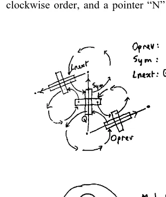
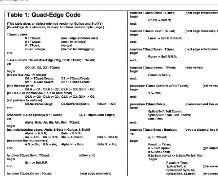
gon structures . Its disadvantage is that storage costs are high by comparison with other methods. It is, however, very easy to implement, especially in an object-oriented environment. Fig. 2 shows the basic structure, with four branches for each edge of the graph being stored, one for each of the adjacent vertices or faces. Table 1 shows the object definition
Ž .
in Delphi Object Pascal . Apart from a pointer to the node or face, each branch has a pointer ARB ŽRot , connecting the four branches together in anti-.
Ž .
clockwise order, and a pointer ANB Next , pointing
Table 1 Quad-Edge code
to the next edge in anticlockwise order around the node or face. Also shown are some of the low-level operations using N and R: ASym,B which moves from the current branch to the branch of the same edge that faces in the other direction;AOprevB which moves to the next branchredge clockwise around the vertexrface associated with the original branch; and
Ž .
ALnextB which equals Sym.Oprev that finds the next branchredge clockwise around the other end of the edge.
To show the simplicity of its use, Figs. 2 and 3 shows the two commands that are used to modify a graph: AMake-EdgeB to create a new edge on a
manifold, and ASpliceB to connectrdisconnect Quad-Edges together. In the simplest case, Splice connects two separateANextB loops, joining the two nodes together, and at the same time splitting the
Ž
ANextB loop around the common face the process could equally well have split theANextB loop around a node, and merged the loops around a face: Splice is its own inverse. See the original paper for more
.
Fig. 3. The Splice operation.
are sufficient to maintain a triangulation network for simple terrain modelling. Work is continuing on
Ž making these operations efficient in secondary rather
.
than just primary storage.
5. Real-world problems with polygon construction
In reality, of course, topology construction in a traditional GIS is a complex operation. It normally consists of a global operation to find all line intersec-tions between the input arcs, followed by various stages of cleanup: removing small dangling arc ends, merging nearby intersections into a single polygon
Ž .
node Pullar, 1994 , etc. Only then may the resulting graph be traversed to create polygons. Additional problems are the detection of self-intersecting arcs, the generation of unwantedAsliver polygonsBif arcs are nearly superimposed, and unconnected islands as
Ž
described above in a tradition GIS, AtopologyB is largely thought of as a polygon construction
prob-. lem .
The nature of the intersection-detection operation indicates a global process rather than an incremental one, and this leads to the necessity of processing the wholeAmapB at once. Thus, most systems are map-sheet based, allowing the processing of a manageable set of data at one time — even if only one arc has been changed from the previous time. Goodchild
Ž1989. has discussed the problem of tiling large spatial data sets. This approach is clearly not appro-priate for a global GIS, which would need an incre-mental algorithm, adding one arc at a time. It should be noted that if the extent of an update can be well defined, then a ApatchB may be created and sewn into the map sheet, thus speeding up the process. All the underlying problems remain, and it is not obvi-ous how to define the update regions. In addition,
Ž .
since features usually arcs cross map-sheet bound-aries, a great deal of effort is required to reconnect features when multiple map sheets are needed. Life would be much easier with an incremental, global topology system! It should be noted here that the maintenance of individual polygon objects only, as in the AShapeB file approach, avoids the problem of map sheet boundaries, and is in this sense AglobalB. However, this approach is intended only for the display of previously defined objects, where topolog-ical structuring has previously been used for bound-ary matching. It is not intended for the maintenance of continually changing structures and relationships. Defining map sheets on the basis of global map coordinates alone ignores the consistency of objects, and in addition breaks the topological connectivity of the global system. A secondary, although relatively minor, problem concerns the co-ordinate system
it-Ž .
self: it must be global not broken into zones , and it Ž
must be continuous throughout unlike latituder
. Ž
longitude . Using direction cosines a vector algebra .
approach , a seamless co-ordinate system simplifies
Ž .
things greatly Fig. 4 . We are storing three
nates for a point instead of two, but there are no Ž
discontinuities in the co-ordinate system as is the case for longitude at plus or minus 1808, or across
.
UTM zones or the equivalent . Good precision is Ž
preserved over the whole globe. Dutton 1989, 1991, .
1996 has extensively explored hierarchical global
Ž .
co-ordinate systems, as have Otoo and Zhu 1993 ,
Ž . Ž .
Fekete 1990 and Goodchild et al. 1991 , and these could well be used for object storage and co-ordinate conversion.
6. Time
GIS as we know them have great difficulty in handling change over time, due largely to the map-sheet approach to topology building. It is not easy to add or remove one feature at a time during the update process. Thus, time is usually treated as a series of Asnapshots,B perhaps at 10-year intervals.
Ž What is needed for updating is an incremental and
.
interactive approach. The problem here arises out of the complexities in the geometry operations, as the incremental update of a planar graph is not a prob-lem.
Outside the traditional polygon map, there are many other applications whose topological structures
Ž .
deserve consideration. Networks roads, rivers pos-sess a topological structure less complete than a
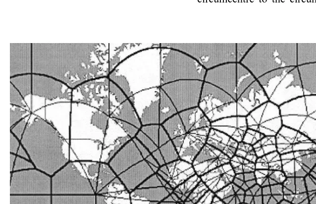
Fig. 5. Orthographic projection, Voronoi cells of points on conti-nent boundaries.
Fig. 6. Regular Voronoi cells on the sphere.
polygon set; in addition, closed loops may not repre-sent regions that need to be named, and unconnected nodes at the ends of arcs are permitted. Point data sets initially may be thought of as having no topolog-ical structure, but they are very often connected into a triangulation. These structures ought to be update-able on an incremental basis also.
Spatial operations that fall outside traditional GIS need to be considered also; in particular, simulation of one form or another where the objects move in space and need dynamic update of their topology. This is a direct continuation of the update problem mentioned above, except that modifications are made as a result of the simulation of the process involved Žthe AfutureB., as opposed to the manual updating of
the known Apast.B A simple example would be
atmospheric modelling, where particles representing packets of air would move around and interact with each other. This can be managed with the triangula-tion structure — in particular the Delaunay triangu-lation, which is the dual of the simple Voronoi diagram. This provides simple rules for determining the neighbouring points to any particular point, and how to update the topological structure as the points
Ž .
move Roos, 1991 . Another approach is that of
Ž .
reactive data structures Van Oosterom, 1993 . In the plane, there are many published examples of algo-rithms for creating the VoronoirDelaunay structure
Ž .
— a good recent example is Devillers 1998 . Okabe
Ž .
et al. 1992 have produced an excellent
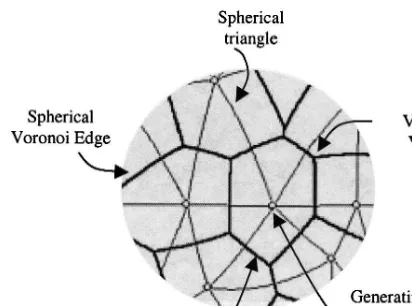
Fig. 7. Portion of the Voronoi diagram and its components on the surface of unit sphere.
the concept of proximal regions has many applica-tions in spatial analysis.
7. A global topological structure
This example of atmospheric modelling naturally brings us to the question of moving our topological
Ž .
structure onto the sphere or ellipsoid . The transfor-mation of a simple planar graph is very easy: take theAexteriorB region, and consider this to be a finite region on the opposite side of the sphere to the viewpoint. For a triangulation, all exterior vertices may be connected to a point on the opposite side of the sphere. This simplifies management of the boundaries of the map, and provides, as Worboys Ž1995 calls it, the. Aperfect 2-spaceB.
Thus, all displayed maps are considered to be projections of the globe — which is quite
reason-Ž able! Voronoi diagrams may be displayed Figs. 5
.
and 6 , as well as the dual Delaunay triangulation. Dynamic point movement may be managed as de-scribed above. The topological structure allows the navigation through the network to locate the enclos-ing triangle of, or the nearest object to, some speci-fied location. Local updates may then be performed to insert or delete an object at that location. Watson Ž1988 and Lukatella 1989 have also developed. Ž . methods for constructing the Voronoi diagram on the
Ž .
sphere, as have Augenbaum and Peskin 1985 .
8. Construction of the Voronoi diagram
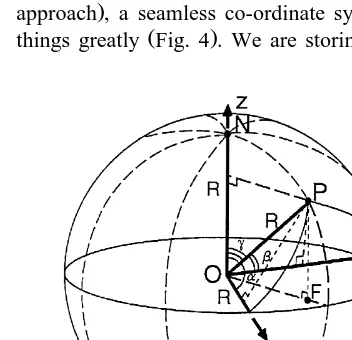
In this section, we briefly describe the construc-tion of the global topology based on the Voronoi diagram on the surface of a sphere. As mentioned in previous sections, we used the direction cosines in three dimensions as the basis of the co-ordinate system for representing the location of the objects on the surface of the sphere. Such a co-ordinate system is earth centred. This system is seamless and allows a continuous representation of the position of the objects on the surface of the sphere, as illustrated in Fig. 7.
4
Consider a collection of N points p , . . . , p1 2 on the surface of a unit sphere. A minimum of four points is needed to initialise the Delaunay triangula-tion and the Voronoi diagram on the sphere. For our purpose, we used six initial points that correspond to
Ž .
Fig. 8. Initialising the Delaunay triangulation. a Choice of six initial points at the intersection of the axes of the coordinate system with the
Ž .
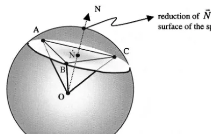
Fig. 9. NXis the circumcentre of the triangle ABC and the point N is the centre of the spherical cap cut by the plan ABC.
the intersection of the axes of the 3D Cartesian co-ordinate system with the surface of the sphere ŽFig. 8 . Using these initial points, we create eight.
Ž
triangles four triangles on the northern hemisphere . and four others on the southern hemisphere . The initially created triangles form a Delaunay triangula-tion on the sphere. This implies that all of the circumcircles of the triangles are empty. These trian-gles cover the surface of the globe and are used as the bases for the construction of the spherical Delau-nay triangulation.
We use the incremental method to create the spherical Delaunay triangulation. This method allows local modification of the structure without recon-struction of the whole topology. The AInsertB and ADeleteB operations for the Delaunay triangulation on the sphere are almost the same as in the planar case, but the optimisation criterion is different. On the surface of the sphere the shortest distance
be-tween two points is defined as the angular distance between these points along the great circle formed by the origin of the sphere and the two points. With this definition, where NX is the circumcentre of the
Ž .
triangle ABC Fig. 9 , the circumradius is the dis-tance between the points A and N on the surface of the sphere measured in radians.
The optimisation procedure on the surface of the sphere consists of comparing of two angular dis-tances. One is the circumradius of the triangle to be tested and the other is the angular distance between the circumcentre of the triangle and a fourth point on the surface of the sphere. If the latter is greater than the circumradius of the triangle, then the fourth point is outside the circumcircle — which implies that the
Ž triangle belongs to the Delaunay triangulation Fig.
.
10 . If the circumcircle of the spherical triangle ABC is not empty then it is not a valid Delaunay triangle. To maintain the Delaunay triangulation in this case, we use the operation called ASwapB to change the diagonal of the spherical quadrilateral formed by the set of four points. The result of the ASwapB opera-tion is two newly created triangles that should be tested again for the Delaunay criterion.
To compute the location of the circumcentre of a spherical triangle we use the following equation
™ ™ ™ ™
ByA = CyA
Ž
.
Ž
.
™
Ns ™ ™ ™ ™ .
Ž .
1<
Ž
ByA.
=Ž
CyA.
<In this equation, = is the vector product and NPN denotes the norm of the vector. A, B, and C are
™
three points on the surface of the unit sphere and N
Ž . Ž .
Fig. 11. Sphere surface partitioning: a Voronoi diagram; b Delaunay triangulation.
is the position vector of the circumcentre of the spherical triangle ABC that passes through the origin™ ™ and is reduced to the surface of the unit sphere. A, B™ and C are the position vectors of the points A, B
Ž .
and C. We can see from the Eq. 1 that since the points A, B, and C can never be on the same
Ž
straight line because they are on the surface of the .
sphere the equation is valid for all the triangles on the sphere.
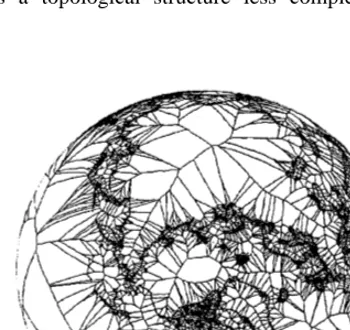
The Voronoi diagram is the dual of the Delaunay triangulation. This implies that we can construct the Voronoi diagram from the Delaunay triangulation and vice versa. This is true for the Voronoi diagram on the plane and on the sphere. In the spherical case, each Voronoi edge is an arc of a great circle between the circumcentres of any two adjacent spherical
tri-Ž .
angles Fig. 7 . For each triangle, we connect its circumcentre to the circumcentres of its three
cent triangles. The resulting diagram is the Voronoi
Ž .
diagram on the sphere Figs. 11 and 12 .
9. Topology vs. attributes
Following topology construction issues, but re-lated to them, are concerns about spatial queries. Within a map-sheet-based system, simple queries are global for the map sheet in most cases: finding all
Ž .
objects houses, polygons, etc. with the desired attributes. This is implicit in a relational database system: a particular table of attributes will be for the whole map. This is not feasible in a true global system: queries must be restricted first by some spatial component, and only then by attribute. The traditional approach would be by some map-sheet structure as described above, with all its complica-tions.
Another alternative would be to use the global topological structure itself: first finding any object within the region of interest, and then expanding outwards to collect everything within that region. The first stage may be performed by walking through the network as described above. For successive queries this walk will usually be relatively short, as work continues on the region of interest. Neverthe-less, this will not always be the case, and some pointer structure may be needed to avoid traversing half the globe to find some initial object within the
Ž .
new region of interest see Gold et al., 1995 . The
Ž .
hierarchical structures of Dutton 1989, 1991, 1996 ,
Ž . Ž .
De Floriani and Puppo 1995 or Jones et al. 1992 could also be used at this stage. The second stage involves a simple graph traversal algorithm such as breadth-first-search, terminating at the region’s boundaries, in order to examine all the objects of
Ž .
interest de Berg et al., 1997 .
Given the premise that a global GIS contains many objects, and that the region of interest is small, this initial step reduces the number of objects exam-ined to a reasonable set. Standard relational queries may then be performed on this reduced set. It should be remembered that typical relational queries are AglobalB in principle: the initial table contains the whole data set, with no spatial limits. Thus, any subsequent query, whether as some form of co-ordinate window, or on some attribute, must start by
examining the whole data set. Clearly, if the global data set is partitioned into map sheets as part of the fundamental data structure this problem is avoided, as queries are addressed to individual sheets. How-ever, if a global data structure is used, with topologi-cal linkages, then the identification of some starting seed object followed by the regional search, as de-scribed above, avoids any requirement to examine the whole data set.
The introduction of time into the picture compli-cates things further. If it is a question of querying the database at some particular point in its updating process, rather than after the completion of some AsnapshotB of the whole system, the approach just described remains unchanged. Queries that are con-strained in space as well as time, and examination of any of the past states of the region, remain a research
Ž .
topic Mioc et al., 1999 . However, if we consider that the number of time states remains small within a local region, then the above approach may be pre-served and the lifespans of the objects may be treated as attributes. This, however, will not preserve the topological structuring at some past time: ques-tions such as AWhen were these two objects adja-cent?Bcannot be handled.
10. The overlay problem
Other questions arise when the traditional tools of polygon overlay and buffer zones are required. These are normally batch operations performed on the whole topological unit — usually the map sheet. In a global system, the objects within the region of inter-est must be extracted by queries, as described above, and then the new topological structure created for that region. This last may be a batch operation, or based on local incremental topology modification. Nevertheless, the effect is to produce a new
topologi-Ž .
cal space or structure for the region of interest, for a particular query. Thus, the utility of global topolog-ical spaces becomes less clear if analysis operations form new local structures that cannot be integrated within the global parent structures.
necessar-ily require the generation of a new topological struc-ture, except for archival purposes.
11. When is a global topological space useful?
This brings us to the key question of this paper: to what extent are global topological structures appro-priate in an ideal system? For our purposes, an ideal
Ž
system would be organised on the globe the sphere .
or ellipsoid , possess very large numbers of map objects, have some topological structure connecting these objects, and be capable of handling frequent small, local map updates. Due to the difficulties encountered in re-joining adjacent separate map sheets, it would be preferable to avoid this problem by having a seamless topology and co-ordinate
sys-Ž
tem for the purpose of this exercise, the problems of paging this data structure into secondary storage will
. be ignored, as being a separate problem .
The primary question concerns the number of basic topological spaces that are required for the project under consideration. These are basically the same thing asAoverlaysB, as they can be thought of
Ž .
as planar more precisely, plane graphs: they may Ž
be connected as in a polygon coverage, or a river
. Ž
network , or disconnected as in point sets or build-.
ings , but they may not conflict with one another by having intersections that are not represented by topo-logical nodes.
Different overlays are used to separate different groups of objects. Each group must be topologically consistent, as just described, but may contain differ-ent classes of features as long as there is no superpo-sition. For example, trees are not usually found on houses, so these may be grouped together in the same overlay, but cars are often found on roads, so
Ž .
these may not be grouped. See Molenaar 1998 for a more detailed treatment of spatial object modelling. However, there is an important consideration: does the operation of classification of a set of objects in a single overlay require that the resulting classes be stored in multiple overlays? At one level they need not: they remain spatially non-overlapping after
be-Ž
ing reclassified think of the reclassification of a .
choropleth map . On another level they may: adja-cency queries may be between buildings of the same
Ž .
type such as police stations , rather than involving
intervening buildings of another type. This issue may be resolved in practice by using more complex oper-ations on the topological space than that of the basic adjacency properties of the simple graph. In our police station example, the stations are not adjacent in terms of the buildings layer, but they are accessi-ble through that layer and the adjacency query may be resolved analytically.
Thus, it appears that the answer to our question depends on how much local topology construction is
Ž .
required for queries overlay, etc. . This in turn depends on the classification of object classes. If there are many types of objects, then the question becomes: do we have a separate global topology for each class? If yes, we can have adjacency type queries within each class, but local batch
construc-Ž
tion for inter-class queries overlay is an inter-class .
query, buffer-zone is not . If we need to classify our
Ž .
objects on the fly, e.g. polygon reclassify and merge then it is not obvious whether the results of this operation are good for local adjacency queries only, or need to be subdivided into their own topological spaces. At first sight it appears that, since the results cannot be superimposed, they can be processed in a single topological space, as with our tentative ap-proach to the police station problem above. One basic rule for topological spaces is that objects in that space may not occupy the same locations: if that can possibly occur, then separate spaces are required. Thus, the primary question is: how many topological spaces are required? Can we make general rules, or do we need to perform semantic analysis for each specific application?
12. Conclusions
Within a single topological space a global system is appropriate. Where multiple topological spaces are
Ž required, then comparisons between them often
.
discrete objects a lot depends on the assumption of two-dimensionality, as with our examples of trees and houses, cars and roads. In both cases, however, there will be the need to extract subsets of the operations in a single topological space in order to answer specific local queries: buffer zones around primary roads only, for example, or the distances between pubs or police stations. These are again one–off operations for specific queries.
The function of a global topological space there-Ž
fore is to contain the objects of a particular spatially .
non-overlapping group. For simple cases, such as simulating atmospheric movement, this should be enough. In other cases, several spaces should be maintained, and local topological structures gener-ated for specific queries. The alternative is to subdi-vide the globe into map-sheets, creating many com-plications.
The starting point for any local operation on a topological space in traditional GIS is to find a map sheet containing some initial location. If a global structure is used, the first step is to find the closest object to the initial location, and then perform an outwards-search to cover the region of interest. This
Ž may be done by a walk through the structure which
.
could be long , or else by adding a simple hierarchi-cal structure to give a close initial estimate. Having obtained a spatially restricted region, local topologi-cal spaces may be generated by overlay or other operations in order to respond to particular queries. A major technical question concerns the storage and retrieval of attribute information: where there are no
Ž .
permanent regions map sheets it is not obvious how to adapt to RDBMS-type structures.
The arguments given above would be appropriate for any appropriate topological structure that can be represented as a graph, possibly stored as Quad-Edges, and can be updated using local operations. Nevertheless, the ideas were organised with the
Ž
Voronoi structure in mind, for example Gold and .
Condal, 1995 , as it has been shown to be maintain-able by local update, can handle time-varying infor-mation, and can readily be generated on the sphere. Thus, the move towards a global GIS would require a locally updateable topological structure, perhaps of that type. It would be necessary to maintain a topo-logical space for each base class of objectsrfields, defined on the basis that duplicate objects may not
exist in the same space at the same location. Topo-logical queries between groups of classes, such as overlay, would require the generation of a temporary topological structure over the region of interest. For some single-space operations, such as flow simula-tion or interpolasimula-tion, this would not be necessary.
Where temporary topological structures are re-quired, it is less clear whether a global topological structure is necessary. On the positive side, it elimi-nates the worries over local co-ordinate systems and map edge-matching. On the negative side, mainte-nance might be excessive if most queries required local temporary topological structures. This would reduce the value of the global structure to data maintenance and extraction of the region of interest. Nevertheless, their benefits for the modelling of simple data types warrant experimentation with the approach, with extension to complex data types and queries if warranted at a later date.
Acknowledgements
This research was supported in part by an NSERCrAIFQ Industrial Research Chair in Geomat-ics at Laval University, Quebec.
References
Augenbaum, J., Peskin, C., 1985. On the construction of the
Ž .
Voronoi mesh on a sphere. J. Comput. Phys. 59 2 , 177–192. Burrough, P.A., 1986. Principles of Geographical Information Systems for Land Resources Assessment. Oxford Univ. Press, Oxford.
de Berg, M., van Kreveld, M., van Oosterum, R., Overmars, M., 1997. Simple traversal of a subdivision without extra storage.
Ž .
Int. J. Geogr. Inf. Sci. 11 4 , 359–373.
De Floriani, L., Puppo, E., 1995. Hierarchical triangulation for multiresolution surface description. ACM Trans. Graphics 14
Ž .4 , 363–411.
De Floriani, L., Falcidieno, B., Nagy, G., Pienovi, C., 1991. On sorting triangles in a Delaunay tessellation. Algorithmica 6
Ž .4 , 522–532.
De Floriani, F., Puppo, E., Magillo, P., 1995. Technical aspects of spatial data. Geographical Information Systems — Materials
Ž .
for a Post-Graduate Course. In: Frank, A. Ed. , GIS Technol. Department of Geoinformation, Technical University of Vi-enna, vol. 2, pp. 395–452.
Dutton, G., 1989. Modelling locational uncertainty via
hierarchi-Ž .
cal tessellation. In: Goodchild, M., Gopal, S. Eds. , Accuracy of Spatial Databases. Taylor & Francis, London, pp. 125–140. Dutton, G., 1991. Polyhedral hierarchical tessellations: the shape
Ž .
of GIS to come. Geo Info Sys. 1 3 , 49–55.
Dutton, G., 1996. Encoding and handling geospatial data with hierarchical triangular meshes. In: Kraak, M.J., Molenaar, M.
ŽEds. , Advances in GIS Research II Proc. SDH7, Delft, The. Ž .
Netherlands . Taylor & Francis, London, pp. 505–518. Fekete, G., 1990. Rendering and managing spherical data with
sphere quadtrees. Proc. IEEE Conf. Visualization ’90. IEEE Computer Society, Los Alamitos, CA, pp. 176–186. Gold, C.M., 1988. PAN Graphs: an aid to GIS analysis. Int. J.
Ž .
Geogr. Inf. Sys. 2 1 , 29–41.
Gold, C.M., 1996. An event-driven approach to spatio-temporal
Ž .
mapping. Geomatica 50 4 , 415–424.
Gold, C.M., Condal, A.R., 1995. A spatial data structure integrat-ing GIS and simulation in a marine environment. Mar. Geod. 18, 213–228.
Gold, C.M., Cormack, S., 1987. Spatially ordered networks and
Ž .
topographic reconstructions. Int. J. Geogr. Inf. Sys. 1 2 , 137–148.
Gold, C.M., Charters, T.D., Ramsden, J., 1977. Automated con-tour mapping using triangular element data structures and an interpolant over each triangular domain. Comput. Graphics 11
Ž .2 , 170–175.
Gold, C.M., Remmele, P., Roos, T., 1995. Voronoi diagrams of
Ž .
line segments made easy. In: Gold, C.M., Robert, J.M. Eds. , Proc. 7th. Canadian Conference on Computational Geometry, Quebec, pp. 223–228.
Goodchild, M.F., 1989. Tiling large geographical databases. Sym-posium on the Design and Implementation of Large Spatial Databases, Santa Barbara, California. Springer, Berlin, pp. 137–146.
Goodchild, M.F., Shiren, Y., Dutton, G., 1991. Spatial Data Representation and Basic Operations for a Triangular
Hierar-chical Data Structure. NCGIA Tech. Paper 91-8, Santa Bar-bara.
Guibas, L., Stolfi, J., 1985. Primitives for the manipulation of general subdivisions, and the computation of Voronoi
dia-Ž .
grams. ACM Trans. Graphics 4 2 , 74–123.
Jones, C.B., Ware, J.M., Bundy, G.L., 1992. Multiscale spatial modelling with triangulated surfaces. Proc. Spatial Data Han-dling 5 vol. 2, pp. 612–621.
Lukatella, H., 1989. Hipparchus data structure: points, lines and regions in a spherical Voronoi grid. Proc. Ninth International
Ž
Symposium on Computer-Assisted Cartography Auto-Carto
.
9 , Baltimore, pp. 164–170.
Mioc, D., Anton, F., Gold, C.M., Moulin, B., 1999.ATime travelB visualization in a dynamic Voronoi data structure. Cartogr.
Ž .
Geogr. Inf. Sci. 26 2 , 99–108.
Molenaar, M., 1998. An Introduction to the Theory of Spatial Object Modelling for GIS. Taylor & Francis, London. Okabe, A., Boots, B., Sugihara, K., 1992. Spatial Tessellations:
Concepts and Applications of Voronoi Diagrams. Wiley, Chichester.
Otoo, E.J., Zhu, H., 1993. Indexing on spherical surfaces using semi-quadcodes. Advances in Spatial Databases. Proc. 3rd International Symposium, SSD’93, Singapore. pp. 510–529. Pullar, D., 1994. A Tractable Approach to Map Overlay. PhD
Dissertation, University of Maine at Orono, 134 pp. Roos, T., 1991. Dynamic Voronoi diagrams. PhD Dissertation,
University of Wurzburg, 213 pp.¨
Sedgewick, R., 1983. Algorithms. Addison-Wesley, Reading, MA, 551 pp.
van Oosterom, P., 1993. Reactive Data Structures for Geographic Information Systems. Oxford Univ. Press, Oxford.
Watson, D.F., 1988. Natural neighbor sorting on the
n-dimen-Ž .
sional sphere. Pattern Recognit. 21 1 , 63–67.