GH2009DC3P004 A4. GH2009DC3P004 A4

(1)

Land Cover Mapping of the Greater

Cape Three Points Area Using Landsat

Remote Sensing Data

February 2012

Y.Q. Wang, Christopher Damon, Glenn Archetto

Donald Robadue and Mark Fenn

THE

UNIVERSITY

of Rhode Island

GRADUATE SCHOOL OF OCEANOGRAPHY

Coastal Resources

(2)

This publication is available electronically on the Coastal Resources Center’s website at

http://www.crc.uri.edu

For more information on the Integrated Coastal and Fisheries Governance project, contact: Coastal Resources Center, University of Rhode Island, Narragansett Bay Campus, 220 South Ferry Road, Narragansett, Rhode Island 02882, USA. Brian Crawford, Director International Programs at [email protected]; Tel: 401-874-6224; Fax: 401-874-6920.

For additional information on partner activities:

WorldFish: http://www.worldfishcenter.org Friends of the Nation: http://www.fonghana.org Hen Mpoano: http://www.henmpoano.org Sustainametrix: http://www.sustainametrix.com

Citation: Wang, Y.Q., Damon, C., Archetto,G., Robadue, D., Fenn, M. (2012) Land Cover Mapping of the Greater Cape Three Points Area Using Landsat Remote Sensing Data. Coastal Resources Center, University of Rhode Island. USAID Integrated Coastal and Fisheries Governance Program for the Western Region of Ghana. 48 pp.

Author contacts: [email protected]; [email protected]

(3)

ii

Acknowledgements

(4)

List of Figures

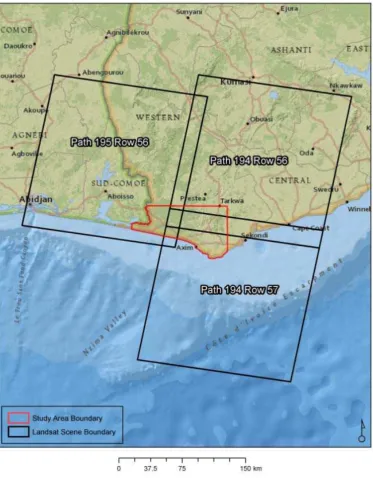
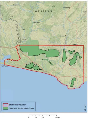
Figure 1: The study area and the coverage of Landsat TM images by path and row numbers . 6 Figure 2: The reserves within the study area ... 7

List of Tables

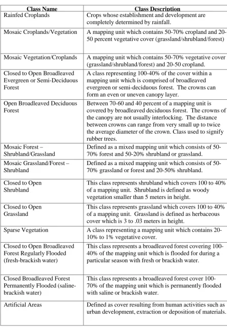
Table 1: Land use and land cover classification for the greater Cape Three Points area, Ghana (adopted from Land Cover Classification System (LCCS)) ... 13

Table 2: Error matrix and accuracy assessment of the land cover classification. ... 15

(5)

4

Introduction

Understanding the spatial arrangement and location of different types of land use and land cover is integral to effectively managing natural, cultural and economic resources. Land use and land cover data allow land managers and other decision makers the ability to observe current conditions on the ground and make informed decisions about how future development should occur. In the past, development was placed without regard as to how it would affect adjacent land uses or whether it was replacing important agricultural, cultural or ecological areas. With the advent of satellite remote sensing and geospatial analysis technologies, land use and land cover maps developed from remotely sensed data have become routine practices in resource management and planning.

Remote sensing has been identified as one of the primary data sources to produce landcover maps that indicate landscape patterns and human development processes (Turner 1990; Coppin and Baure, 1996; Griffith et al., 2003; Rogan et al., 2002; Turner et al., 2003; Wilson and Sader, 2002; Wang et al., 2003). Landsat type of remote sensing data has been used in coastal applications for decades (Munday and Alfoldi, 1979; Bukata et al., 1988; Ritchie et al., 1990). The multispectral capabilities of the data allow observation and measurement of biophysical characteristics of coastal habitats (Colwell, 1983), and the multi-temporal capabilities allow tracking of changes in these characteristics over time (Wang and Moskovits, 2001).

Remote sensing derived land use and land cover maps are especially important for developing countries where landscape changes occur quickly and often encroach into previously

undisturbed areas (Awusabo-Asare et al., 2005). Some of the major pressures driving the loss of natural areas include timber extraction, agricultural development and infrastructure

development (Fuller, 2006). These catalysts are reflected in the specific concerns for western Ghana which include increased oil exploration, illegal gold mining operations, the

proliferation of rubber plantations, and the loss of mangrove habitat. Coupling land use and land cover mapping with other planning techniques can mitigate the impacts of land use change and provide a mechanism to effectively balance resource protection with competing development interests.

One particular advantage that remote sensing can provide for inventory and monitoring of protected lands is the information for understanding the past and current status, the changes occurred under different impacting factors and management practices, the trends of changes in comparison with adjacent areas and implications of changes on ecosystem functions (e.g., Hansen and DeFries, 2007a,b). This is reflected as a component of the

(6)

system develop from the United Nations Land Cover Classification system (LCCS) (Arino et al., 2007). The LCCS is a hierarchical a priori classification scheme built to provide a broad, yet flexible standardized classification system that would be effective at providing global scale land cover information (Di Gregorio, 2000). This system emerged from the

AFRICOVER mapping project where broad based classification systems were needed to map the varied landscapes found throughout Africa. The LCCS allows for a robust description of land cover types and is compatible with future land use analyses while providing flexibility to meet additional needs which may arise.

The Study Area

(7)

6

(8)

(9)

8

Methods

The procedures of the mapping exercise included to:

1. Obtain the best available Landsat multispectral data from the available USGS

archives. We made efforts to obtain and use the best appropriate data available taking into account percent cloud cover and overall data quality.

2. Initial land cover mapping via stratified image classification process. This exercise included pre-processing of the Landsat images in order to develop workable data for the focused study area.

3. Obtain field reference data for verification and improvement of the initial classification results.

4. Prepare a comprehensive set of land-cover maps of the study area that meets the needs for landscape characterization (e.g., patchness, connectivity, configuration and

composition), habitat analysis, and assessment of carbon storing capacity of the study area.

Data

Base data for this project was acquired from the USGS Landsat program. The satellite images were obtained from the Landsat 5 Thematic Mapper (TM) sensor. The images for the eastern portion of the study extent (Path 194/Row56-57) were acquired on 1/15/2002 and the western portion image was acquired on 2/23/2000 (Path 195/Row56) (Figure 1). Landsat 5 TM images possess a spatial resolution of 30 meters with seven spectral bands ranging from visible to infrared portion of the spectrum. The images were processed and subset to the extent of the study area as defined.

Classification Procedures

Due to the lack of previous comparable data, a pre-classification stratification was not performed; instead the images were subset into areas of similar land use or cloud cover to limit differences in spectral signatures. These subset images were processed by unsupervised classifications using ERDAS Imagine® software system. The resulting spectral clusters were assigned the land use and land cover categories according to the descriptions of the LCCS (Table 1). We use the fifteen land cover classes to this land cover mapping exercise

(Appendix I).

Field Checking and Referencing

Guided by the local ecologists and field experts, the project team members (Wang and

Damon) conducted field checking and referencing for the verification of the initial land cover map by the classification process. Prior fieldwork a set of referencing maps was developed. The sample points were created using ArcGIS software system and were randomly assigned throughout the study area for the land cover categories initially classified. The maps of referencing points were developed for both the Landsat TM images and the initial land use and land cover classification maps for the field comparison purpose (Appendix II).

Due to time constraints and the large geographic area being sampled, 80 of the 400 points generated were actually visited during the fieldwork time. A Trimble YMA-FYS6AS-00 Yuma was employed for field navigation and photographic documentation.

(10)

for the documentation of the surrounding landscape characteristics and land use and land cover types (Appendix III). The photographs were taken from the four cardinal directions. Those field visited points were then used to adjust the previous classification to improve overall accuracy.

Final Land Use and Land Cover Map

We conducted the final classification improvement by referencing the field observations and verifications and by using a pre-classification stratification. This process reduced spectral disparities in the subset images. Once the classification was complete, an accuracy

assessment was performed to determine the accuracy of the land cover map.

Accuracy Assessment

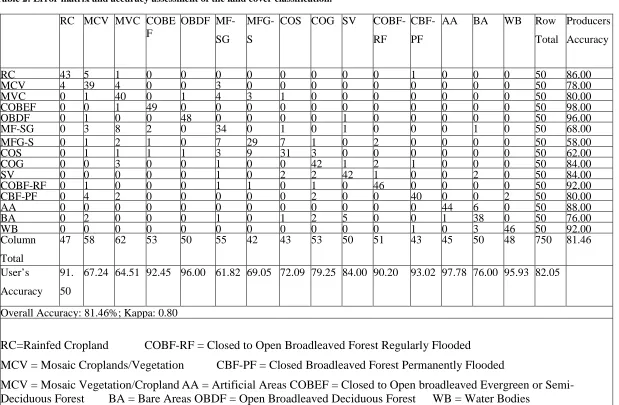
The error matrix was developed to report classification accuracy. An error matrix is a square array of numbers laid out in rows and columns that express the number of sample units assigned to a particular category relative to the actual category as verified in the field. The columns normally represent the reference data, while the rows indicate the classification generated from remotely sensed data. The overall accuracy of the classification map is determined by dividing the total correct pixels (sum of the major diagonal) by the total number of pixels in the error matrix (N ).

Computing the accuracy of individual categories is more complex because there are different choices of dividing the number of correct pixels in the category by the total number of pixels in the corresponding row or column. The total number of correct pixels in a category is divided by the total number of pixels of that category as derived from the reference data (i.e., the column total). This statistic indicates the probability of a reference pixel being correctly classified and is a measure of omission error, or error of exclusion. This statistic is also called the producer’s accuracy because the producer (the analyst) of the classification is interested in how well a certain area can be classified. If the total number of correct pixels in a category is divided by the total number of pixels that were actually classified in that category, the result is a measure of commission error, or error of inclusion. This measure, called the user’s

accuracy or reliability, is the probability that a pixel classified on the map actually represents

that category on the ground.

(11)

10

Results

The set of final composite of land use and land cover maps for the study area was created in the scale of 1:60,000. The page-size examples of the final maps are enclosed in the report in the Appendix IV. While a full compilation of land use and land cover classes and their areas can be found in Table 3, some of the results are summarized below.

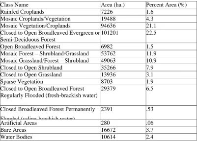
1. The mapping result indicated that the Closed to Open Broadleaved Deciduous Forest category was the largest land cover type at 101,201 hectares.

2. The Mosaic Vegetation/Cropland was the second largest land cover type at 94,636 hectares.

3. The Closed to Open Broadleaved Deciduous Forest was mostly located in large and contiguous areas aside with natural reserves.

4. The Mosaic Vegetation/Cropland was the most widespread land cover type representing the landscape of local farming practices.

5. Freshwater wetlands, as a component of the Open to Closed Broadleaved Regularly Flooded, were prevalent on the landscape with an area of 29,379 hectares.

6. The coastal wetlands were about 2,391 hectares as a component of the category of Closed Broadleaved Permanently Flooded.

7. Much of the freshwater wetlands occurred towards the western half of the study region, occurring along the coast and along the Comoe River.

8. The Mosaic Forest-Shrubland/Grassland category covered the area of 53,762 hectares. 9. The Mosaic Grassland/Forest-Shrubland covered the area of 49,063 hectares. These

land cover areas were interspersed throughout the heavily cleared regions of the study area.

10. The Open Broadleaved DeciduousForest, which was used as a proxy for capturing rubber trees, covered the area of 6,892 hectares, most of which was located in large, contiguous areas in the Cape Three Points region.

The accuracy assessment reported that the land cover maps achieved an overall accuracy of 81.2% with a kappa of .80. Homogeneous classes with unique spectral signatures had higher individual accuracies overall, while classes with mixed land use types tended to have lower accuracies. Overall, the categories of Closed to Open Broadleaved Deciduous Forest, Open

Broadleaved Deciduous Forest, Closed to Open Broadleaved Forest Regularly Flooded, Closed Broadleaved Permanently Flooded, Artificial Areas and Water Bodies had producers

accuracies above 90%, while classes such as Mosaic Croplands/Vegetation, Mosaic

Vegetation/Crops and Mosaic Forest-Shrubland Grassland had lower accuracies because of

(12)

Discussion

Optical remote sensing relies on the accurate retrieval of radiation emitted from the sun by satellite sensors positioned hundreds of kilometers above the earths surface (Kerr, 2003). A major error which can occur during this process is interference by atmospheric

contamination. This type of error can be caused by the ozone, water vapor, aerosols, sand storms or other atmospheric processes (Kerr, 2003). In equatorial regions, cloud and haze coverage are common during the rainy season, which coincides with the collection of this data. This type of interference causes variance in spectral signatures and creates shadows which further degrade the response from ground features. Steps such as sub- setting similar areas and attempts at radiometric correction were taken to lessen the impact of this error, but overall its effects are difficult to remove (Kerr, 2003). This may give insight into the lack of consistency in accuracy among classes. Large, contiguous classes with homogenous or unique signatures such as Closed to Broadleaved Deciduous Forest and Closed to Open

Broadleaved Forest Regularly Flooded were easier to identify and subset out, leading to

higher accuracies. Conversely, mosaic classes which had very similar spectral signatures and occurred in highly fragmented matrixes had lower accuracies. These classes were difficult to isolate from other similar classes and the effects of cloud cover and haze often limited

differences in reflectance, hindering the ability to accurately identify them.

Sub-setting also introduced some artifacts of the classification to the final thematic image. While sub-setting was necessary to control the effects of haze and cloud cover, the frequent use of this technique can cause inconsistency between adjacent areas. Such effects can be witnessed in the areas surrounding wetlands near the coast. Due to the increased wetness during the rainy season and spectral interference caused by cloud cover, areas which consisted of agricultural land uses were being associated with wetlands. Sub-setting was used to correct for this, but some artifacts of this process are still visible.

Another inconsistency which could have resulted in classification error was temporal differences between the western and eastern Landsat images used to perform this analysis. The images were taken approximately one year apart, and were unable to be mosaicked together due to differences in cloud cover and spectral signatures. These scenes represented the best data for the coastal region of Ghana that was freely available through the USGS Landsat Earth Explorer data center. Lacking the ability to combine these two scenes, there were classified separately and mosaicked after the analysis was complete.

Finally, the method of accuracy analysis could also be a source of error. The GPS data collected during field work in Ghana was unable to be used in the accuracy assessment due to their use in correcting the preliminary classification and there were limited high spatial resolution images available to be used as a ground truth. These leads to the accuracy

assessment being performed as the classes were understood by the analyst. This process was impaired by lack of spectral uniformity within classes. Classes which were large and

(13)

12

Conclusion

(14)

Table 1: Land use and land cover classification for the greater Cape Three Points area, Ghana (adopted

from Land Cover Classification System (LCCS))

Class Name Class Description

Rainfed Croplands Crops whose establishment and development are completely determined by rainfall.

Mosaic Croplands/Vegetation A mapping unit which contains 50-70% cropland and 20-50 percent vegetative cover (grassland/shrubland/forest) Mosaic Vegetation/Croplands A mapping unit which contains 50-70% vegetative cover

(grassland/shrubland/forest) and 20-50 cropland. Closed to Open Broadleaved

Evergreen or Semi-Deciduous Forest

A class representing 100-40% of the cover within a mapping unit which is comprised of broadleaved evergreen or semi-deciduous forest. The crowns can form an even or uneven canopy layer.

Open Broadleaved Deciduous Forest

Between 70-60 and 40 percent of a mapping unit is covered by broadleaved deciduous forest. The crowns of the canopy are not usually interlocking. The distance between crowns can range from very small up to twice the average diameter of the crown. Class used to signify rubber trees.

Mosaic Forest – Shrubland/Grassland

Defined as a mixed mapping unit which consists of 50-70% forest and 50-20% shrubland or grassland. Mosaic Grassland/Forest –

Shrubland

Defined as a mixed mapping unit which consists of 50-70% grassland or forest and 20-50% shrubland. Closed to Open

Shrubland

This class represents shrubland which covers 100 to 40% of a mapping unit. Shrubland is defined as woody vegetation smaller than 5 meters in height.

Closed to Open Grassland

This class represents grassland which covers 100 to 40% of a mapping unit. Grassland is defined as herbaceous cover which is 3 to .03 meters in height.

Sparse Vegetation A class representing a mapping unit which contains 20-10% to 1% vegetative cover.

Closed to Open Broadleaved Forest Regularly Flooded (fresh-brackish water)

This class represents a broadleaved forest covering 100-40% of the mapping unit which is flooded for during a particular season with fresh or brackish water.

Closed Broadleaved Forest Permanently Flooded (saline- brackish water)

This class represents a broadleaved forest cover 100-70% of the mapping unit which is permanently flooded with saline or brackish water.

(15)

14

Class Name Class Description

Bare Areas A class representing areas which are not covered by vegetation or artificial cover. Can be comprised of rocky or sandy areas.

(16)

Table 2: Error matrix and accuracy assessment of the land cover classification.

Overall Accuracy: 81.46%; Kappa: 0.80

RC=Rainfed Cropland COBF-RF = Closed to Open Broadleaved Forest Regularly Flooded

MCV = Mosaic Croplands/Vegetation CBF-PF = Closed Broadleaved Forest Permanently Flooded

MCV = Mosaic Vegetation/Cropland AA = Artificial Areas COBEF = Closed to Open broadleaved Evergreen or Semi-Deciduous Forest BA = Bare Areas OBDF = Open Broadleaved Deciduous Forest WB = Water Bodies

(17)

16 Table 3: Land use and land cover mapping results.

Class Name Area (ha.) Percent Area (%)

Rainfed Croplands 7226 1.6

Mosaic Croplands/Vegetation 19488 4.3

Mosaic Vegetation/Croplands 94636 21.1

Closed to Open Broadleaved Evergreen or Semi-Deciduous Forest

101201 22.5

Open Broadleaved Forest 6982 1.5

Mosaic Forest – Shrubland/Grassland 53762 11.9 Mosaic Grassland/Forest – Shrubland 49063 10.9

Closed to Open Shrubland 35266 7.9

Closed to Open Grassland 13936 3.1

Sparse Vegetation 8703 1.9

(18)

References

Awusabo-Asare, K., A. Kumi-Kyereme and M.J. White, 2005. Urbanization, Development, and Environmental Quality: Insights from Coastal Ghana. IUSSP 2005 Sessions: S903: Urbanization, Environment, and Development

Bukata, R.P., J.H. Jerome, and J.E. Bruton, 1988. Particulate concentrations in Lake St. Clair as recorded by a shipborne multispectral optical monitoring system, Remote Sensing of

Environment, 25: 201–229.

Colwell, R.N., 1983, Manual of Remote Sensing, 2nd edition. American Society of Photogrammetry, Falls Church, VA.

Coppin, P.R. and M.E. Bauer, 1996. Digital change detection in forest ecosystem with remotely sensed imagery, Remote Sensing Review, 13: 207-234.

Fuller, D.O. 2006. Tropical Forest Monitoring and Remote Sensing: A New Era of Transparency in Forest Governance?. Singapore Journal of Tropical Geography 27, 15- 29

Griffith, J.A., Stehman, S.V., Sohl, T.L. and T.R. Loveland, 2003. Detecting trends in landscape pattern metrics over a 20-year period using a sampling-based monitoring programme. International Journal of Remote Sensing 24:175-181.

Hansen, A.J. and R. DeFries, 2007a. Land use change around nature reserves: Implications for sustaining biodiversity. Ecological Applications, 17(4) 972-973.

Hansen, A.J. and R. DeFries. 2007b. Ecological mechanisms linking protected areas to surrounding lands. Ecological Applications 17(4), 974-988.

Kerr, J.T., M. Ostrovsky, 2003. From Space to Species: Ecological Applications for Remote Sensing. TRENDS in Ecology and Evolution 18 (6)

Munday, J.C., Jr. and AIfoldi, T.T., 1979, Landsat test of diffuse refl ectance models for aquatic suspended solids measurements, Remote Sensing of Environment, 8: 169–183.

Ritchie, J.C., C.M. Cooper, and F.R. Shiebe, 1990, The relationship of MSS and TM digital data with suspended sediments, chlorophyll and temperature in Moon Lake, Mississipi, Remote Sensing

of Environment, 33: 137–148.

Rogan, J., J. Franklin and D.A. Roberts, 2002. A comparison of methods for monitoring multitemporal vegetation change using Thematic Mapper imagery, Remote Sensing of Environment, 80: 143-156.

Turner, M.G., 1990, Spatial and Temporal Analysis of Landscape Patterns, Landscape Ecology 4:21-30.

Turner, W., S. Spector, N. Gardiner, M. Fladeland, E. Sterling and M. Steininger, 2003. Remote sensing for biodiversity science and conservation, TRENDS in Ecology and Evolution, 18(3): 306-314.

Wang, Y., G. Bonynge, J. Nugranad, M. Traber, A. Ngusaru, J. Tobey, L. Hale, R. Bowen and V. Makota, 2003. Remote sensing of Mangrove Change Along the Tanzania Coast, Marine Geodesy, 26(1-2):35-48.

Wang, Y. and D.K. Moskovits, 2001. Tracking fragmentation of natural communities and changes in land cover: Applications of Landsat data for conservation in an urban landscape (Chicago Wilderness), Conservation Biology, 15(4): 835–843.

(19)

18

Appendix I. The Land Cover Classification System (LCCS)

The U.N. Land Cover Classification System is a hierarchical a priori classification system. It was developed in order to provide a broad, flexible yet standardized classification system that would be effective in providing land use land cover information for the world. The current Land Cover Classification System (LCCS) emerged from the Africover project where a broad based classification system needed to map the varied landscapes found in Africa. The

problem with previous attempts at large scale a prior classification systems was that in order to cover vastly different landscapes, they required large numbers of classes which often have very similar class boundaries. This leads to a lack of standardization as different users may have different interpretations of these thresholds. Those which attempt to use broad, generic classes have a high level of standardization but often lack the specificity to meet the needs of multiple end users. In order to meet its design goal of fulfilling the needs of a wide variety of users and mapping vast geographic areas, the LCCS was designed with a two phase

classification system which provides a flexible, modular framework.

The first phase of the LCCS system is the Dichotomous phase. This is where a pixels major land cover type is distinguished. There are eight different land cover types in this phase which are categorized by using three criteria; presence of vegetation, edaphic condition and

artificiality of cover. The eight classes encompass all possible land types and include Cultivated and Managed Terrestrial Areas, Natural and Semi-Natural Terrestrial Vegetation, Cultivated Aquatic or Regularly Flooded areas, Natural and Semi- Natural Aquatic or Regularly Flooded Vegetation, Artificial Surfaces and Associated Areas, Bare Areas,

Artificial Water Bodies, Snow and Ice and Natural Water Bodies, Snow and Ice. This phase is followed by a Modular-Hierarchical phase in which land cover classes are created by

combining pre-defined modifiers. This allows users to choose the most relevant classifiers for their study areas without losing the benefits of an a priori system. There are two main types of classifiers which can be added to the eight main land cover classes. The first are

environmental attributes which influence land cover but are not actual features within it. These include things such as climate, landform, altitude and soils. The second classifier is Specific Technical Attributes which allows users to utilize specific classifiers which may only apply to their research. Examples of this could be soil type in bare areas or crop type in cultivated areas.

For the purpose of this classification, the classes which will be used to identify land use and land cover have already been predefined as those selected by the Globcover project. This project aims to provide global land use land cover data by using an automated system with predefined thresholds. In order to do this, Globcover uses the ESA’s Envisat environmental satellite which takes 300 meter spatial resolution images. From here, the satellite data is delineated into more than 20 unique land cover classes. Classes which will be included in the study were those previously identified by the Globcover project. Overall, there were 14 classes included in the study area after the Globcover data was subset to the study areas borders.

(20)

open shrubland, closed to open grassland, and sparse vegetation. The next category, artificial and bare surfaces are defined by the lack of vegetative cover. Artificial surfaces are defined as cover resulting from human activities. This includes urban development, transportation, surface mining and waste dumps. Bare areas are those which have neither vegetative nor artificial cover. This class comprises of rocky outcrops, bare soil and sand. Finally, water bodies and flood lands include all natural water bodies which are covered by water for a period of the year. Water bodies are defined as permanently flooded natural water bodies such as the ocean, lakes, ponds or rivers. Flooded lands are separated into two classes; closed to open broadleaved forest regularly flooded (fresh-brackish water) and closed broadleaved forest permanently flooded (saline-brackish water). Both of these classes are defined by the presence of water which inundates these areas for considerable amounts of time. The soil type and plant communities reflect the influence of water and these classes could include

mangroves, wooded wetlands or bog areas.

The classes themselves lend an understanding of what the general classification boundaries are, but due to the modular nature of this system, the classifiers have an important function in delineation which may not be apparent. In order to better understand the

Modular-Hierarchical terms which will be used in this study, they will be briefly described here. The structural terms of open and closed describe the amount of landcover being occupied by that land cover class within the minimum mapping unit. Closed describes a class which occupies greater than 60 – 70 percent of the total area of a minimal mapping unit (MMU), open describes a class which occupies less than 70 percent but more than 20 percent MMU and sparse describes a class which occupies less than 20 percent but more than 1 percent of the MMU. Next, the term mosaic describes a class in which two or three individual land cover types share space within one MMU. There are two possible scenarios in which this type of land cover class becomes possible. The first is when each class is a spatially separate entity, such as agricultural fields within a forest. The second is when these classes are in an intricate mixture such as rainfed cultivated field with interlaced woodlands. When dealing with this scenario, the sequence of class names within the mixed mapping unit represents the

dominance of that class in the landscape. In order for a class to be considered for naming within a mixed mapping unit, it must occupy more than 20 percent of the unit.

Any class which has over 50 percent coverage in the mapping unit is considered to be

dominant and is named first. Finally, the classifier rainfed can be used to modify agricultural classes to define the irrigation method used which can have significant influence on which crops will be planted. Rainfed describes a crop which lacks artificial irrigation and whose establishment and growing season is entirely dependent on rainfall.

(21)

20

(22)

(23)

(24)

(25)

(26)

(27)

(28)

(29)

(30)

(31)

30

Appendix Ill. Field photos for mapped land use and land cover

Appendix IV. Land Use and Land Cover Maps

(39)

(40)

(41)

(42)

(43)

(44)

(45)

(46)

(47)

(48)