El e c t ro n ic
Jo ur n
a l o
f
P r
o b
a b i l i t y
Vol. 12 (2007), Paper no. 23, pages 661–683.
Journal URL
http://www.math.washington.edu/~ejpecp/
Occupation laws for some time-nonhomogeneous
Markov chains
∗Zach Dietz
Department of Mathematics Tulane University
6823 St. Charles Ave., New Orleans, LA 70118 [email protected]
Sunder Sethuraman Department of Mathematics
Iowa State University 396 Carver Hall, Ames, IA 50011
Abstract
We consider finite-state time-nonhomogeneous Markov chains whose transition matrix at timenisI+G/nζ whereGis a “generator” matrix, that isG(i, j)>0 fori, j distinct, and G(i, i) =−Pk6=iG(i, k), andζ >0 is a strength parameter. In these chains, as time grows, the positions are less and less likely to change, and so form simple models of age-dependent time-reinforcing schemes. These chains, however, exhibit a trichotomy of occupation behav-iors depending on parameters.
We show that the average occupation or empirical distribution vector up to time n, when variously 0< ζ <1,ζ >1 orζ= 1, converges in probability to a unique “stationary” vector νG, converges in law to a nontrivial mixture of point measures, or converges in law to a distributionµG with no atoms and full support on a simplex respectively, asn ↑ ∞. This last type of limit can be interpreted as a sort of “spreading” between the cases 0< ζ <1 and ζ >1.
In particular, whenGis appropriately chosen,µG is a Dirichlet distribution, reminiscent of results in P´olya urns.
Key words: laws of large numbers, nonhomogeneous, Markov, occupation, reinforcement, Dirichlet distribution.
1
Introduction and Results
In this article, we study asymptotic occupation laws for a class of finite space time-nonhomogeneous Markov chains where, as time increases, positions are less likely to change. Although these chains feature simple age-dependent time-reinforcing dynamics, some different, perhaps unexpected, asymptotic occupation behaviors emerge depending on parameters. A spe-cific case, as in Example 1.1, was first introduced in Gantert [7] in connection with the analysis of certain simulated annealing laws of large numbers phenomena.
Example 1.1. Suppose there are only two states 1 and 2, and that the chain moves between the
two locations in the following way: At large timesn, the chain switches places with probability
c/n, and stays put with complementary probability 1−c/n for c >0. The chain, as it ages, is less inclined to leave its spot, but nonetheless switches infinitely often. It can be seen that the probability of being in state 1 tends to 1/2 regardless of the initial distribution. One may ask, however, how the average occupation, or frequency up to time n of state 1, n−1Pni=111(Xi), behaves asymptotically as n ↑ ∞. For this example, it was shown in [7] and Ex. 4.7.1 [27], surprisingly, that the frequency could not converge to a constant, or even more generally con-verge in probability to a random variable, without further investigation of the limit properties. However, a quick consequence of our results is that the frequency of state 1 converges in law to the Beta(c, c) distribution (Theorem 1.4).
More specifically, we consider a general version of this scheme with m≥2 possible locations, and moving and staying probabilities G(i, j)/nζ and 1−Pk6=iG(i, k)/nζ from i → j 6= i and
i→ i respectively at time nwhere G ={G(i, j)} is an m×m matrix and ζ > 0 is a strength parameter. After observing the location probability vector,hPG,ζπ (Xn =k) : 1≤k≤mi, tends
to a vector νG,π,ζ, as n ↑ ∞, which depends on G, ζ, and initial probability π when ζ > 1, but does not depend on ζ and π, νG,π,ζ = νG, when ζ ≤ 1 (Theorem 1.1), the results on the limit of the average occupation or empirical distribution vector,n−1Pn
i=1h11(Xi), . . . ,1m(Xi)i, asn↑ ∞, separate into three cases depending on whether 0< ζ <1,ζ = 1, or ζ >1.
When 0< ζ < 1, following [7], the empirical distribution vector is seen to converge to νG in probability; and when more specifically 0< ζ <1/2, this convergence is proved to be a.s. When
ζ >1, as there are only a finite number of switches, the position eventually stabilizes and the empirical distribution vector converges in law to a mixture of point measures (Theorem 1.2).
Our main results are when ζ = 1. In this case, we show the empirical distribution vector converges in law to a non-atomic distributionµG, with full support on a simplex, identified by its moments (Theorems 1.3 and 1.5). When, in particular, G takes form G(i, j) = θj for all
i6=j, that is when the transititions into a statej are constant,µG takes the form of a Dirichlet distribution with parameters{θj} (Theorem 1.4). The proofs of these statements follow by the method of moments, and some surgeries of the paths.
The heuristic, with respect to the asymptotic empirical distribution behavior, is that when 0< ζ <1 the chance of switching is strong and sufficient mixing gives a deterministic limit, but whenζ >1 there is little movement and the chain gets stuck in finite time. The boundary case
ζ = 1 is the intermediate “spreading” situation leading to non-atomic limits. For example, with respect to Ex. 1.1, when the switching probability at time nis c/nζ, the Beta(c, c) limit when
0 0.1 0.2 0.3 0.4 0.5 0.6 0.7 0.8 0.9 1 0
0.5 1 1.5 2 2.5 3 3.5 4
x
density
c = 10.0 c = 1.0 c = 0.1
Figure 1: Beta(c, c) occupation law of state 1 in Ex. 1.1.
limit of state 1 when 0 < ζ < 1, and the fair mixture of point measures at 0 and 1, the limit when ζ >1 and starting at random (cf. Fig. 1).
In the literature, there are only a few results on laws of large numbers-type asymptotics for time-nonhomogeneous Markov chains, often related to simulated annealing and Metropolis algorithms which can be viewed in terms of a generalized model where ζ = ζ(i, j) is a non-negative function. These results relate to the cases, “maxζ(i, j) < 1” or when the “landscape function” has a unique minimum, for which the average occupation or empirical distribution vector limits are constant [7], Ch. 7 [27], [10]. See also Ch. 1 [15], [18],[26]; and texts [5], [13],[14] for more on nonhomogeneous Markov chains. In this light, the non-degenerate limits
µG found here seem to be novel objects. In terms of simulated annealing, these limits suggest a more complicated asymptotic empirical distribution picture at the “critical” cooling schedule when ζ(i, j) = 1 for some pairsi, j in the state space with respect to general “landscapes.”
The advent of Dirichlet limits, when G is chosen appropriately, seems of particular interest, given similar results for limit color-frequencies in P´olya urns [4], [8], as it hints at an even larger role for Dirichlet measures in related but different “reinforcement”-type models (see [16], [21], [20], and references therein, for more on urn and reinforcement schemes). In this context, the set of “spreading” limitsµG in Theorem 1.3, in which Dirichlet measures are but a subset, appears intriguing as well (cf. Remarks 1.4, 1.5 and Fig. 2).
In another vein, although different, Ex. 1.1 seems not so far from the case of independent Bernoulli trials with success probability 1/n at the nth trial. For such trials much is known about the spacings between successes, and connections to GEM random allocation models and Poisson-Dirichlet measures [25], [1], [2], [3], [22], [23].
We also mention, in a different, neighbor setting, some interesting but distinct frequency limits have been shown for arrays of time-homogeneous Markov sequences where the transition matrix
Pn for the nth row converges to a limit matrix P [6], [9], Section 5.3 [14]; see also [19] which comments on some “metastability” concerns.
a generator with nonzero entries if M(i, j) > 0 for 1 ≤i, j ≤ m distinct, and M(i, i) < 0 for 1≤i≤m.
To avoid technicalities, e.g. with reducibility, we work with the following matrices,
G =
G∈Rm×m:G is a generator matrix with nonzero entries
,
although extensions should be possible for a larger class. For G ∈ G, let n(G, ζ) = ⌈max1≤i≤m|G(i, i)|1/ζ⌉, and define forζ >0
PnG,ζ =
I for 1≤n≤n(G, ζ)
I+G/nζ forn≥n(G, ζ) + 1
where I is the m×m identity matrix. Then, for all n≥1, PnG,ζ is ensured to be a stochastic matrix.
Letπ be a distribution on Σ, and letPG,ζπ be the (nonhomogeneous) Markov measure on the
sequence space ΣN
with Borel sets B(ΣN
) corresponding to initial distribution π and transition kernels {PnG,ζ}. That is, with respect to the coordinate process, X = hX0, X1, . . .i, we have
PG,ζπ (X0 =i) =π(i) and the Markov property
PG,ζ
π (Xn+1 =j|X0, X1, . . . , Xn−1, Xn=i) =PnG,ζ+1(i, j)
for alli, j∈Σ andn≥0. Our convention then is thatPnG,ζ+1controls “transitions” between times
n and n+ 1. Let also EG,ζπ be expectation with respect to PG,ζπ . More generally, Eµ denotes
expectation with respect to measureµ.
Define the average occupation or empirical distribution vector, forn≥1,
Zn=hZ1,n,· · ·, Zm,ni where Zk,n = 1
n
n X
i=1
1k(Xi)
for 1≤k≤m. Then,Zn is an element of them−1-dimensional simplex,
∆m =
x:
m X
i=1
xi = 1,0≤xi≤1 for 1≤i≤m
.
The first result is on convergence of the position of the process. For G ∈ G, let νG be the
stationary vector corresponding to G (of the associated continuous time homogeneous Markov chain), that is the unique left eigenvector, with positive entries, normalized to unit sum, of the eigenvalue 0.
Theorem 1.1. For G∈G,ζ >0, initial distributionπ, and k∈Σ,
lim n→∞
PG,ζ
π Xn=k
= νG,π,ζ(k)
where νG,π,ζ is a probability vector on Σdepending in general on ζ, G, and π. When0< ζ ≤1,
Remark 1.1. Forζ >1, with only finitely many moves, actuallyXnconverges a.s. to a random variable with distributionνG,π,ζ. Also, νG,π,ζ is explicit whenG=VGDGVG−1 is diagonalizable with DG diagonal and DG(i, i) = λiG, the ith eigenvalue of G, for 1≤ i≤ m. By calculation,
νG,π,ζ =πtQn≥1P
G,ζ
n =πtVGD′VG−1 withD′ diagonal andD′(i, i) =Qn≥n(G,ζ)+1(1 +λGi /nζ). We now consider the casesζ 6= 1 with respect to average occupation or empirical distribution vector limits. Let i be the basis vector i = h0, . . . ,0,1,0, . . . ,0i ∈ ∆m with a 1 in the ith component andδi be the point measure at ifor 1≤i≤m.
Theorem 1.2. Let G∈G, and π be an initial distribution. UnderPG,ζπ , asn↑ ∞, we have that
Zn −→ νG
converges to the vector νG in probability when 0 < ζ <1; when more specifically 0 < ζ < 1/2,
this convergence isPG,ζπ -a.s.
However, when ζ >1,Zn converges PG,ζπ a.s. to a random variable, and
lim n→∞Zn
d =
m X
i=1
νG,π,ζ(i)δi .
Remark 1.2. Simulations suggest that actually a.s. convergence might hold also on the range
1/2≤ζ <1 (with worse convergence rates as ζ ↑1).
Let now γ1, . . . , γm ≥ 0, be integers such that ¯γ = Pmi=1γi ≥ 1. Define the list A = {ai : 1≤i≤¯γ}={1, . . . ,1
| {z } γ1
,2, . . . ,2 | {z }
γ2
, . . . , m, . . . , m
| {z } γm
}. LetS(γ1, . . . , γm) be the ¯γ! permutations ofA,
although there are only γ ¯γ
1,γ2,···,γm
distinct permutations; that is, each permutation appears Qm
k=1γk! times.
Note also, for G ∈ G, being a generator matrix, all eigenvalues of G have non-positive real
parts (indeed, I +G/k is a stochastic matrix for k large; then, by Perron-Frobenius, the real parts of its eigenvalues satisfy−1≤1 + Re(λG
i )/k≤1, yielding the non-positivity), and so the resolvent (xI−G)−1 is well defined for x≥1.
We now come to our main results on the average occupation or empirical distribution vector limits whenζ = 1
Theorem 1.3. Forζ = 1,G∈G, and initial distributionπ, we have under PG,ζπ as n↑ ∞ that
Zn −→d µG
where µG is a measure on the simplex ∆m characterized by its moments: For 1≤i≤m,
EµG xi = lim n→∞
EG,ζ
π Zi,n = νG(i),
and for integersγ1, . . . , γm≥0 whenγ¯≥2,
EµG
xγ1
1 · · ·xγmm
= lim n→∞
EG,ζ
π
Zγ1
1,n· · ·Zm,nγm
= 1 ¯
γ
X
σ∈S(γ1,...,γm)
νG(σ1) ¯
γ−1
Y
i=1
iI−G
−1
Remark 1.3. However, as in Ex. 1.1 and [7], when ζ = 1 as above, Zn cannot converge in probability to a random variable (as the tail field∩nσ{Xn, Xn+1, . . .}is trivial by Theorem 1.2.13
and Proposition 1.2.4 [15] and (2.3), but the limit distributionµG is not a point measure by say Theorem 1.5 below). This is in contrast to P´olya urns where the color frequencies converge a.s.
We now consider a particular matrix under which µG is a Dirichlet distribution. For
θ1, . . . , θm>0, define
Θ =
θ1−θ¯ θ2 θ3 · · · θm
θ1 θ2−θ¯ θ3 · · · θm ..
. ... . .. · · · ...
θ1 θ2 θ3 · · · θm−θ¯
where ¯θ = Pml=1θl. It is clear Θ ∈ G. Recall identification of the Dirichlet distribution by its density and moments; see [17], [24] for more on these distributions. Namely, the Dirichlet distribution on the simplex ∆mwith parametersθ1, . . . , θm (abbreviated as Dir(θ1, . . . , θm)) has density
Γ(¯θ) Γ(θ1)· · ·Γ(θm)
xθ1−1
1 · · ·xθmm −1. The moments with respect to integers γ1, . . . , γm ≥0 with ¯γ ≥1 are
E
xγ1
1 · · ·xγmm
= Qm
i=1θi(θi+ 1)· · ·(θi+γi−1) Qγ¯−1
i=0(¯θ+i)
, (1.1)
where we take θi(θi+ 1)· · ·(θi+γi−1) = 1 when γi = 0.
Theorem 1.4. We have µΘ= Dir(θ1, . . . , θm).
Remark 1.4. Moreover, by comparing the first few moments in Theorem 1.3 with (1.1), one
can checkµG is not a Dirichlet measure for manyG’s withm≥3. However, whenm= 2, then anyGtakes the form of Θ withθ1=G(2,1) andθ2=G(1,2), and soµG= Dir(G(2,1), G(1,2)).
We now characterize the measures {µG :G ∈G} as “spreading” measures different from the limits when 0< ζ <1 and ζ >1.
Theorem 1.5. Let G∈G. Then, (1) µG(U) >0 for any non-empty open set U ⊂∆m. Also,
(2)µG has no atoms.
Remark 1.5. We suspect better estimates in the proof of Theorem 1.5 will show µG is in fact
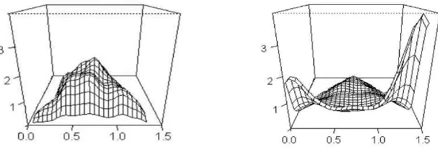
mutually absolutely continuous with respect to Lebesgue measure on ∆m. Of course, in this case, it would be of interest to find the density ofµG. Meanwhile, we give two histograms, found by calculating 1000 sample averages, each on a run of time-length 10000 starting at random on Σ at time n(G,1) (= 3,1 respectively), in Figure 2 of the empirical density whenm= 3 and G
takes forms
Gleft=
−3 1 2
2 −3 1 1 2 −3
, and Gright=
−.4 .2 .2
.3 −.6 .3
.5 .5 −1
Figure 2: EmpiricalµG densities underGleft and Grightrespectively.
To help visualize plots, ∆3 is mapped to the plane by linear transformation f(x) =
x1f(h1,0,0i) +x2f(h0,1,0i) +x3f(h0,0,1i) where f(h1,0,0i) = h√2,0i, f(h0,1,0i) = h0,0i
and f(0,0,1) = √2h1/2,√3/2i. The map maintains a distance √2 between the transformed vertices.
We now comment on the plan of the paper. The proofs of Theorems 1.1 and 1.2, 1.3, 1.4, and 1.5 (1) and (2) are in sections 2,3,4, 5, and 6 respectively. These sections do not depend structurally on each other.
2
Proofs of Theorems 1.1 and 1.2
We first recall some results for nonhomogeneous Markov chains in the literature. For a stochastic matrixP on Σ, define the “contraction coefficient”
c(P) = max x,y
1 2
X
z
P(x, z)−P(y, z)
= 1−min x,y
X
z min
P(x, z), P(y, z)
(2.1)
The following is implied by Theorem 4.5.1 [27].
Proposition 2.1. LetXnbe a time-nonhomogeneous Markov chain onΣconnected by transition
matrices{Pn}with corresponding stationary distributions{νn}. Suppose, for some n0 ≥1, that
∞ Y
n=k
c(Pn) = 0 for all k≥n0, and
∞ X
n=n0
kνn−νn+1kVar<∞. (2.2)
Then, ν = limn→∞νn exists, and, starting from any initial distribution π, we have for each
k∈Σ that
lim
A version of the following is stated in Section 2 [7] as a consequence of results (1.2.22) and Theorem 1.2.23 in [15].
Proposition 2.2. Given the setting of Proposition 2.1, suppose (2.2) is satisfied for some n0≥
1. Define cn= maxn0≤i≤nc(Pi) for n≥n0. Let also π be any initial distribution, and f be any functionf : Σ→R. Then, we have convergence, as n→ ∞,
1
n
n X
i=1
f(Xi) → Eν[f]
in the following senses:
(i) In probability, when limn→∞n(1−cn) =∞.
(ii) a.s. whenPn≥n02−n(1−c2n)−2 <∞ (with convention the sum diverges if c2n = 1 for an
n≥n0).
Proof of Theorem 1.1. We first consider whenζ >1. In this case there are only a finite number of movements by Borel-Cantelli sincePn≥1PG,ζπ (Xn6=Xn+1)≤CP
n≥1n−ζ <∞. Hence there
is a time of last movementN <∞ a.s. Then, limn→∞Xn=XN a.s., and, for k∈Σ, the limit distributionνG,π,ζ is defined and given byPG,ζπ (XN =k) =νG,π,ζ(k).
When 0< ζ ≤1, as G∈G, by calculation with (2.1),c(PnG,ζ) = 1−CG/nζ, with respect to a
constantCG >0, for all n ≥n0(G, ζ) for an index n0(G, ζ) > n(G, ζ) large enough. Then, for
k≥n0(G, ζ),
Y
n≥k
1−CG
nζ
= 0. (2.3)
Since for n ≥n0(G, ζ), νGtP G,ζ
n =νGt(I −G/nζ) = νGt, the last condition of Proposition 2.1 is trivially satisfied, and hence the result follows.
Proof of Theorem 1.2. When ζ >1, as mentioned in the proof of Theorem 1.1, there are only a finite number of moves a.s., and so a.s. limn→∞Zn = Pmk=11[XN=k]k concentrates on basis
vectors {k}. Hence, as defined in proof of Theorem 1.1, PG,ζπ (XN = k) = νG,π,ζ(k), and the
result follows.
When 0< ζ < 1, we apply Proposition 2.2 and follow the method in [7]. First, recalling the proof of Theorem 1.1, (2.2) holds, andcn= maxn0(G,ζ)≤i≤nc(P
G,ζ
i ) = 1−CG/nζ for a constant
CG>0 and n≥n0(G, ζ). Then, n(1−cn) =CGn1−ζ ↑ ∞to give the probability convergence in part (i). For a.s. convergence in part (ii) when 0< ζ <1/2, note
X
n≥n0(G,ζ)
1 2n(1−c
2n)2 =
X
n≥n0(G,ζ)
1 2n(C
G/(2n)ζ)2
= X
n≥n0(G,ζ)
1
C2
G(21−2ζ)n
< ∞.
3
Proof of Theorem 1.3.
In this section, as ζ = 1 is fixed, we suppress notational dependence on ζ. Also, as Zn takes values on the compact set ∆m, the weak convergence in Theorem 1.3 follows by convergence of the moments.
Lemma 3.1. For G∈G, 1≤k≤m, and initial distribution π,
Proof. From Theorem 1.1, and Cesaro convergence,
lim
We now turn to the joint moment limits in several steps, and will assume in the following that
γ1, . . . , γm ≥0 with ¯γ ≥2. The first step is an “ordering of terms.”
The next lemma replaces the initial measure withνG. LetPi,jG = Qj
Lemma 3.3. For G∈Gand initial distribution π, we have
which differs from the second expression in (3.1) by at most
X
which vanishes by Theorem 1.1.
We now focus on a useful class of diagonalizable matrices
G∗ =
diagonalizableG∈Gbelong toG∗. The relevance of this class, in the subsequent arguments, is
that forG∈G∗ the resolvent (xI−G)−1 exists forx≥1.
ForG∈G∗, letVGbe the matrix of eigenvectors andDGbe a diagonal matrix with
correspond-ing eigenvalue entries DG(i, i) =λGi so that G=VGDGVG−1. Define also for 1≤s, t, k≤m,
g(k;s, t) = VG(s, k)VG−1(k, t).
We also denote for a1, . . . , am ∈C, the diagonal matrix Diag(a·) with ith diagonal entry ai for 1 ≤i≤m. We also extend the definitions ofPG
n and Pi,jG to G∈ G∗ with the same formulas. In the following, we use the principal value of the complex logarithm, and the usual convention
Proof. Straightforwardly,
and note by the simple estimate
Definingν(s;i, j) = exp(c(s;i, j) +d(s;i, j)) gives after multiplying out that
The next lemma estimates a “boundary” contribution.
Lemma 3.5. For G∈G, continuous on [ǫ,1]2 for fixed s, t, and Riemann convergence, we have
Lemma 3.7. For G∈G∗ and σ ∈S(γ1, . . . , γm),
and fǫ is uniformly bounded over ǫas
|fǫ| ≤ f¯ = 1{0<x1≤x2≤···≤xγ¯≤1}
The right-hand bound is integrable: Indeed, by Tonelli’s Lemma and induction, we have
Z
Hence, the lemma follows by dominated convergence and Fubini’s Theorem.
Lemma 3.8. For G∈G∗ and σ ∈S(γ1, . . . , γm),
Proof. By induction, the integral equals
to finish the identification.
At this point, by straightforwardly combining the previous lemmas, we have proved Theorem 1.3 for G ∈ G diagonalizable. The method in extending to non-diagonalizable generators is
accomplished by approximating with suitable “lower” and “upper” diagonal matrices.
Lemma 3.9. For G∈G,
lim n→∞
X
σ∈S(γ1,...,γm)
νG(σ1)
n¯γ
n−¯γ+1
X
i1=1
n−¯γ+2
X
i2>i1
· · · n X
iγ>i¯ ¯γ−1
¯
γ−1
Y
l=1
PilG+1,il+1(σl, σl+1)
= 1 ¯
γ
X
σ∈S(γ1,...,γm) νG(σ1)
¯
γ−1
Y
l=1
lI−G
−1
(σl, σl+1). (3.2)
Proof. For an m×m matrix A, let G[A] =G+A. Let k · kM be the matrix norm kAkM =
max{|A(s, t)| : 1 ≤ s, t ≤ m}. Now, for small ǫ > 0, choose matrices A1 and A2 with
non-negative entries so thatkA1kM,kA2kM < ǫ,I +G[−A1]/l, I+G[A2]/l have positive entries for
allllarge enough, andG[−A1], G[A2]∈G∗: This last condition can be met as (1) the spectrum
varies continuously with respect to the matrix norm k · kM (cf. Appendix D [12]), and (2)
diagonalizable real matrices are dense (cf. Theorem 1 [11]).
Then, for s, t ∈Σ, and l large enough, we have 0< (I +G[−A1]/l)(s, t) ≤(I +G/l)(s, t) ≤
(I+G[A2]/l)(s, t). Hence, fori≤j withilarge enough,
PG[−A1]
i,j (s, t) ≤ Pi,jG(s, t) ≤ Pi,jG[A2](s, t).
By Lemmas 3.5, 3.6, 3.7 and 3.8, the left-side of (3.2), that is in terms of liminf and limsup, is bounded below and above by
X
σ∈S(γ1,...,γm)
1 ¯
γνG(σ1)
¯
γ−1
Y
l=1
lI−G[−A1]
−1
(σl, σl+1),
and
X
σ∈S(γ1,...,γm) 1 ¯
γνG(σ1)
¯
γ−1
Y
l=1
lI −G[A2]
−1
(σl, σl+1)
respectively. On the other hand, forσ ∈S(γ1, . . . , γm), both
¯
γ−1
Y
l=1
lI−G[−A1]−1(σl, σl+1), ¯
γ−1
Y
l=1
lI−G[A2]−1(σl, σl+1) → ¯
γ−1
Y
l=1
lI−G−1(σl, σl+1)
asǫ→0, completing the proof.
4
Proof of Theorem 1.4
Lemma 4.1. The stationary distribution νΘ is given by νΘ(l) =θl/θ¯for l∈Σ.
Also, for 2≤l≤¯γ, let Fl be the m×m matrix with entries
Fl(j, k) =
θk fork6=j
θj+l−1 for k=j.
Then,
lI −Θ −1
= 1
l(l+ ¯θ)Fl+1.
Proof. The form of νΘ follows by inspection. For the second statement, writeFl+1 =lI + ˆΘ
where the matrix ˆΘ hasith column equal toθi(1, . . . ,1)t. Then, also Θ = ˆΘ−θI¯ . As (1, . . . ,1)t is an eigenvector of Θ with eigenvalue 0, we see (lI −Θ)(lI + ˆΘ) = (l2 +lθ¯)I finishing the proof.
The next statement is an immediate corollary of Theorem 1.3 and Lemma 4.1.
Lemma 4.2. The µΘ-moments satisfy EµΘ[xi] =θi/θ¯for 1≤i≤m and, when ¯γ ≥2,
EµΘ
m Y
i=1
xγii
= X
σ∈S(γ1,...,γm) νΘ(σ1)
1 ¯
γ
¯
γ−1
Y
l=1
lI−Θ −1
(σl, σl+1)
= X
σ∈S(γ1,...,γm) θσ1
Qγ¯
l=2Fl(σl−1, σl)
¯
γ!Q¯γl=0−1(¯θ+l) .
We now evaluate the last expression of Lemma 4.2 by first specifying of the value ofσγ¯. Recall,
by conventionθl· · ·(θl+γl−1) = 1 when γl= 0 for 1≤l≤m.
Lemma 4.3. For ¯γ ≥2 and 1≤k≤m,
X
σ∈S(γ1,...,γm)
σγ¯=k
θσ1
¯
γ Y
l=2
Fl(σl−1, σl) = γk(¯γ−1)! m Y
l=1
θl· · ·(θl+γl−1). (4.1)
Proof. The proof will be by induction on ¯γ.
Base Step: γ¯ = 2. If γk = 1 and γi = 1 for i6= k, the left and right-sides of (4.1) both equal
θiF2(i, k) =θiθk. Ifγk = 2, then the left and right-sides of (4.1) equal 2θkF2(k, k) = 2θk(θk+ 1).
Induction Step. Without loss of generality and to ease notation, letk= 1. Then, by specifying the next-to-last elementσγ¯−1, and simple counting, we have
X
σ∈S(γ1,...,γm)
σγ¯=1
θσ1
¯
γ Y
l=2
Fl(σl, σl−1) = γ1(θ1+ ¯γ−1)
X
σ∈S(γ1−1,...,γm)
σ¯γ−1=1
θσ1
¯
γ−1
Y
l=2
Fl(σl, σl−1)
+ m X
j=2
γ1θ1
X
σ∈S(γ1−1,...,γm)
σ¯γ−1=j
θσ1
¯
γ−1
Y
l=2
We now use induction to evaluate the right-side above as
θ1· · ·(θ1+γ1−2)
m Y
i=2
θi· · ·(θi+γi−1)
×
γ1(θ1+ ¯γ−1)(γ1−1)(¯γ−2)! +
m X
j=2
γ1θ1γj(¯γ −2)!
= θ1· · ·(θ1+γ1−2)
m Y
i=2
θi· · ·(θi+γi−1)
×
γ1(θ1+ ¯γ−1)(γ1−1)(¯γ−2)! +γ1θ1(¯γ−γ1)(¯γ−2)!
= θ1· · ·(θ1+γ1−2)
m Y
i=2
θi· · ·(θi+γi−1)
×γ1(¯γ−2)!
(θ1+γ1−1)(¯γ−1)
= γ1(¯γ−1)!
m Y
l=1
θl· · ·(θl+γl−1).
By now adding over 1≤k≤m in the previous lemma, we finish the proof of Theorem 1.4.
Lemma 4.4. When γ¯≥2,
X
σ∈S(γ1,...,γm)
θσ1
Qγ¯
l=2Fl(σl−1, σl)
¯
γ!Q¯γl=0−1(¯θ+l) = Qm
l=1θl· · ·(θl+γl−1) Q¯γ−1
l=0(¯θ+l)
.
Proof.
X
σ∈S(γ1,...,γm) θσ1
Q¯γ
l=2Fl(σl−1, σl) ¯
γ!Qγl¯=0−1(¯θ+l) = m X
k=1
X
σ∈S(γ1,...,γm)
σ¯γ=k
θσ1
Qγ¯
l=2Fl(σl−1, σl) ¯
γ!Q¯γl=0−1(¯θ+l)
= Pm
k=1γk(¯γ−1)!
¯
γ!
Qm
l=1θl· · ·(θl+γl−1)
Q¯γ−1
l=0(¯θ+l)
= Qm
l=1θl· · ·(θl+γl−1) Q¯γ−1
l=0(¯θ+l)
.
5
Proof of Theorem 1.5 (1)
Let p=hp1, . . . , pmi ∈Int∆m be a point in the simplex with pi > 0 for 1≤i≤m. For ǫ >0 small, letB(p, ǫ)⊂Int∆m be a ball with radius ǫand centerp. To prove Theorem 1.5 (1), it is enough to show for all largen the lower bound
PGπ
Zn∈B(p, ǫ)
To this end, let ¯p0 = 0 and ¯pi = Pil=1pl for 1 ≤ i ≤ m. Also, define, for 1 ≤ k ≤ l,
6
Proof of Theorem 1.5 (2)
The proof of Theorem 1.5 (2) follows from the next two propositions.
Proof. From Theorem 1.3, momentsαl,k =EµG[(xl)k] satisfyαl,k+1= (I−G/k)−1(l, l)αl,k for 1≤l≤m and k≥1. By the inverse adjoint formula, for large k,
I −G/k
−1
(l, l) = 1−
1
k(Tr(G)−G(l, l)) 1−Tr(G)/k +O(k
−2) = 1 +G(l, l)
k +O(k
−2).
As G∈G,G(l, l) <0. Hence, αl,k vanishes at polynomial rate αl,k ∼kG(l,l). In particular, as
µG({l})≤EµG[(xl)k]→0 ask→ ∞, the pointlcannot be an atom of the limit distribution. Fix for the remainder p∈∆m\ {1, . . . ,m}, and define ˇp= min{pi :pi >0,1≤i≤m} >0. Let also 0< δ <p/ˇ 2, and consider B(p, δ) ={x∈∆m :|p−x|< δ}.
Proposition 6.2. For G∈G, there is a constant C=C(G,p, m) such that
µG
B(p, δ)
≤ C log
ˇ
p+ 2δ
ˇ
p−δ
.
Before proving Proposition 6.2, we will need some notation and lemmas. We will say a “switch” occurs at time 1< k≤nin the sequenceωn=hω1, . . . , ωni ∈Σnifωk−16=ωk. For 0≤j ≤n−1, let
T(j) =
ωn:ωn has exactly j switches
.
Note asp∈∆m\ {1, . . . ,m}at least two coordinates of pare positive. Then, asδ <p/ˇ 2, when (1/n)Pni=1h11(ωi), . . . ,1m(ωi)i ∈B(p, δ), at least one switch is inωn.
For j ≥ 1 and a path in T(j), let α1, . . . , αj denote the j switch times in the sequence; let also θ1, . . . , θj+1 be the j + 1 locations visited by the sequence. We now partition {ωn :
(1/n)Pni=1h11(ωi), . . . ,1m(ωi)i ∈ B(p, δ)} ∩T(j) into non-empty sets Aj(U,V) where U = hU1, . . . , Uj−1i and V = hV1, . . . , Vj+1i denote possible switch times (up to the j−1st switch
time) and visit locations respectively:
Aj(U,V) =
ωn:ωn∈T(j),1 n
n X
i=1
h11(ωi), . . . ,1m(ωi)i ∈B(p, δ),
αi =Ui, θk=Vk for 1≤i≤j−1,1≤k≤j+ 1
.
In this decomposition, paths in Aj(U,V) are in 1 : 1 correspondence with jth switch times
αj–the only feature allowed to vary.
Now, for each set Aj(U,V), we define a path η(j,U,V) = hη1, . . . , ηni where the last jth switch is “removed,”
ηl=
V1 for 1≤l < U1
Vk forUk−1≤l < Uk,2≤k≤j−1
Vj forUj−1≤l≤n.
Note that the sequenceη(j,U,V) belongs to T(j−1), can be obtained no matter the location
with pair hU1, . . . , Uj−1i and hV1, . . . , Vji. In particular, recalling Xn1 = hX1, . . . , Xni denotes the coordinate sequence up to timen, we have
X
U,V PG
π
Xn1 =η(j,U,V)
≤ m PG
π
Xn1 ∈T(j−1)
(6.1)
where the sum is over allU,V corresponding to the decomposition into setsAj(U,V) of {ωn: (1/n)Pni=1h11(ωi), . . . ,1m(ωi)i ∈B(p, δ)} ∩T(j).
The next lemma estimates the location of the last switch time αj, and the size of the set
Aj(U,V). The proof is deferred to the end.
Lemma 6.1. On Aj(U,V), we have ⌈n(ˇp−δ) + 1⌉ ≤αj. Also,|Aj(U,V)| ≤ ⌊2nδ+ 1⌋.
A consequence of these bounds on the position and cardinality of αj’s associated to a fixed setAj(U,V), is that
′
X 1
Uj ≤
⌈n(ˇp+δ)+2⌉ X
k=⌈n(ˇp−δ)+1⌉ 1
k ≤ log
ˇ
p+δ+ 3/n
ˇ
p−δ
(6.2)
whereP′ refers to adding over all last switch times Uj associated to paths inAj(U,V). Let now ˆG= max{|G(i, j)|: 1≤i, j ≤m}.
Lemma 6.2. For ωn∈A
j(U,V) such thatαj =Uj, and all largen, we have
PG
π
Xn1 =ωn
≤ Gˆ(ˇp/2)
−2 ˆG
Uj
PG
π
Xn=η(j,U,V)
. (6.3)
Proof. The path η(j,U,V) differs from ωn only in that there is no switch at time U
j. Hence,
PG
π Xn=ωn
PG
π Xn=η(j,U,V)
=
G(Vj, Vj+1)
Uj(1 +G(Vj, Vj)/Uj) n Y
l=Uj+1
1 +G(Vj+1, Vj+1)/l
1 +G(Vj, Vj)/l
.
Now boundingG(Vj, Vj+1)≤Gˆ, 1 +G(Vj+1, Vj+1)/l≤1, 1 +G(Vj, Vj)/l≥1−G/lˆ , and noting
Uj ≥n(ˇp−δ) + 1 (by Lemma 6.1), −ln(1−x)≤2x forx >0 small, andδ <p/ˇ 2, give for large
n,
G(Vj, Vj+1)
1 +G(Vj, Vj)/Uj n Y
l=Uj+1
1 +G(Vj+1, Vj+1)/l
1 +G(Vj, Vj)/l
≤Gˆ
n n(ˇp−δ)
2 ˆG
≤Gˆ(ˇp/2)−2 ˆG.
Proof of Proposition 6.2. By decomposing over number of switchesj and on the structure of the paths withjswitches, estimates (6.3), (6.2), comment (6.1), andPjPG
π Xn∈T(j−1)
we have for all largen,
The proposition follows by taking limit onn, and weak convergence.
Proof of Lemma 6.1. For a path ωn ∈ Aj(U,V) and 1 ≤ k ≤ j+ 1, let τk be the number
Then, from the deduction just after (6.4), we have
n(ˇp−δ) ≤ n max
giving the first statement.
For the second statement, note that −njτj +Pτji=1−1(nji −nji + 1) (with convention the sum vanishes whenτj = 1) is independent of paths inAj(U,V) being some combination of{Ui : 1≤
i ≤ j−1}. Hence, with k = j in (6.4), we observe αj = njτj + 1 takes on at most ⌊2nδ+ 1⌋ distinct values. The result now follows as paths in Aj(U,V) are in 1 : 1 correspondence with last switch timesαj.
Acknowledgement. We thank M. Bal´azs and J. Pitman for helpful communications, and
References
[1] Arratia, R. (1998) On the central role of scale invariant Poisson processes on (0,∞). Micro-surveys in discrete probability (Princeton, NJ, 1997), 21-41, DIMACS Ser. Discrete Math. Theoret. Comput. Sci., 41, Amer. Math. Soc., Providence, RI MR1630407
[2] Arratia, R., Barbour, A. D., Tavar´e, S. (1999) On Poisson-Dirichlet limits for random de-composable combinatorial structures.Combin. Probab. Comput. 8 193–208. MR1702562
[3] Arratia, R., Barbour, A. D., Tavar´e, S. (2003) Logarithmic Combinatorial Structures: A Probabilistic Approach EMS Monographs in Mathematics. European Mathematical Society (EMS), Z¨urich. MR2032426
[4] Athreya, K.B. (1969) On a characteristic property of P´olya’s urn.Studia Sci. Math. Hungar.
4 31-35. MR0247643
[5] Br´emaud, P. (1999) Markov chains. Gibbs fields, Monte Carlo simulation, and Queues.
Texts in Applied Mathematics 31. Springer-Verlag, New York MR1689633
[6] Dobrushin, R. (1953) Limit theorems for Markov chains with two states. (Russian) Izv. Adad. Nauk SSSR17:4 291-330. MR0058150
[7] Gantert, N. (1990) Laws of large numbers for the annealing algorithm. Stochastic Process. Appl.35309-313. MR1067115
[8] Gouet, R. (1997) Strong convergence of proportions in a multicolor P´olya urn. J. Appl. Probab.34426-435. MR1447347
[9] Hanen, A. (1963) Th´eor`emes limites pour une suite de chaˆınes de Markov. Ann. Inst. H. Poincar´e18197-301. MR0168017
[10] Hannig, J., Chong, E.K.P., Kulkarni, S.R. (2006) Relative frequencies of generalized simu-lated annealing.Math. Oper. Res. 31199-216. MR2205528
[11] Hartfiel, D. J.(1995) Dense sets of diagonalizable matrices. Proc. Amer. Math. Soc. 123
1669–1672. MR1264813
[12] Horn, R. A., Johnson, C. R. (1990)Matrix Analysis.Corrected reprint of the 1985 original. Cambridge University Press, Cambridge. MR1084815
[13] Isaacson, D.L., and Madsen, R.W. (1976) Markov Chains. Theory and Applications. John Wiley and Sons, New York. MR0407991
[14] Iosifescu, M. (1980)Finite Markov Processes and Their Applications.John Wiley and Sons, New York. MR0587116
[15] Iosifescu, M., and Theodorescu, R. (1969)Random Processes and Learning.Springer-Verlag, Berlin. MR0293704
[16] Kotz, S., Balakrishnan, N. (1997) Advances in urn models during the past two decades. In
[17] Kotz, S., Balakrishnan, N., Johnson, N.L. (2000) Continuous Multivariate Distributions
John Wiley and Sons, New York.
[18] Liu, Wen, Liu, Guoxin (1995) A class of strong laws for functionals of countable nonhomo-geneous Markov chains.Stat. and Prob. Letters22 87-96. MR1327733
[19] Miclo, L. (1998) Sur les temps d’occupations des processus de Markov finis inhomog`enes `a basse temp´erature. (French) Stochastics Stochastics Rep.6365-137. MR1639780
[20] Del Moral, P., Miclo, L. (2006) Self-interacting Markov chains.Stoch. Anal. Appl. 24 615-660. MR2220075
[21] Pemantle, R. (2007) A survey of random processes with reinforcement.Probability Surveys
4 1-79. MR2282181
[22] Pitman, J. (1996) Some developments of the Blackwell-MacQueen urn scheme. InStatistics, Probability and Game Theory; Papers in honor of David Blackwell, Ed. T.S. Ferguson et al. Institute of Mathematical Statistics Lecture Notes-Monograph Series 30 245-267. MR1481784
[23] Pitman, J. (2006)Combinatorial stochastic processes.Lecture Notes in Mathematics, 1875
Springer-Verlag, Berlin. MR2245368
[24] Sethuraman, J. (1994) A constructive definition of Dirichlet priors.Statist. Sinica4639–650. MR1309433
[25] Vervaat, W. (1972) Success Epochs in Bernoulli Trials. Math. Centre Tracts, Amsterdam MR0328989
[26] Wen, Liu, Weiguo, Yang (1996) An extension of Shannon-McMillan theorem and some limit properties for nonhomogeneous Markov chains. Stoch. Proc. Appl.61129-145. MR1378852