SOME RESULTS REGARDING
THE ULTRASONIC CAVITATION
by
Alina Bărbulescu and Vasile Mârza
Abstract: The aim of this paper is to prove the existence of the material erosion in ultrasonic field and to measure the intensity of the cavitation phenomenon. We give a mathematical model for the voltage induced by the cavitation.
Keywords: ultrasonic cavitation, erosion, voltage
1. PRELIMINARIES
When an acoustic wave propagates through a liquid containing microscopic gas inclusions, these ''nucleation sites'' can be mechanically activated, at which point they spawn free bubbles which then undergo highly energetic volume pulsations. Associated with these pulsations is a broad range of linear and nonlinear mechanical behavior, the nature of which will primarily depend on the acoustic pressure amplitude and the equilibrium bubble. This activity, which is termed acoustic cavitation, is often accompanied with other physical (erosion, unpassivation and emulsification) or chemical (the production of radical and excited species; single electron transfer) interactions.
We chose to study the mechanical erosion in the ultrasonic field and some mathematical aspects related to the electric field produced by the cavitation bubbles. Rayleigh gave a mechanical explanation of the materials destruction by cavitation. Other scientists consider that these damages are produced by chemical or electrical effects; but, it seems that they are the results of the mechanical pressure inside the bubble.
Plesset and Elis proved that the plastic deformation appears everywhere where a cavitation exists. Their studies bring to the conclusion that the chemical action can't be the primary cause of the erosion.
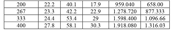
In order to determine the effect of the ultrasound on the propagation medium, the spectral analysis was made, before and after ultrasonic treatment. It was also weighted material put in the sonication bath and it was determined the intensity of the ultrasonic action on the propagation medium.
2. EXPERIMENTAL RESULTS
We used an ultrasound generator of the tip I.U.S. - 150 and of maximum power 180W, with three degrees of electrical power: I: 80W, II: 120W, III: 180W.
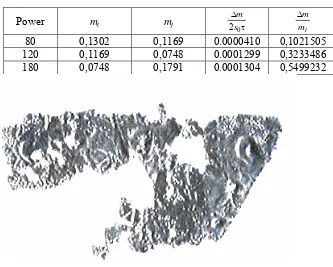
In the sonication bath was introduced, in water, an aluminium foil, weighed before and after the experiment. The results obtained after 30 minutes, for each power are given in the table 1, where:
-
m
i is the initial mass of the aluminium foil (g),-
m
jis the mass of the aluminium foil, after the sonication (g), - τ is the sonication time, in minutes (in our case, 30 minutes), -∆
m
=
m
j−
m
i,-
s
0is the foil surface (cm2). [image:2.595.164.497.323.590.2]It can be seen that, if the power is greater, the loss of the mass, also increases. For the second case, the mass variation is 3.83 times greater than in the first case and in the third case, the lost mass is 5.38 times greater than in the fist case.
Table 1. The aluminium erosion
Power mi mj τ
∆
0 2s
m
i
m m
∆
80 0,1302 0,1169 0.0000410 0,1021505
120 0,1169 0,0748 0.0001299 0,3233486
180 0,0748 0,1791 0.0001304 0,5499232
In order to determine the caloric power we have following formula is used:
τ
=
Q
P
c (1)where:
-τ is the time of the ultrasounds application,
- Q is the quantity of the heat obtained by the ultrasounds propagation in the studied liquid:
Q
=
C
(
θ
−
θ
0)
, (2)- θ is the equilibrium temperature in the calorimeter, -
θ
0is the initial temperature of the calorimeter, - C is the caloric capacity of the calorimeter.We introduced in the calorimeter a piece of copper, with the mass m = 0.1027Kg, with the specific heat c =393.86J/KgK and the initial temperature θ =1000 C. The final temperature was θ1=33.30 C.
The quantity of the waste heat by the copper is equal with absorbed heat by the calorimeter if the calorimeter contains the same water quantity as during the measurement of the caloric power given by the ultrasounds. Thus:
(
θ
−
θ
0)
=
m
Cuc
Cu(
100
−
θ
)
⇒
C
. (3)(
)
K
J
.
.
.
.
.
C
243
2
22
3
33
3
33
100
86
393
0127
0
=
−
⋅
−
⋅
=
.Using the ultrasonic generator of 1MHz, we measured the temperature increasing of the ultrasonically treated liquid. We've determined the temperature variations and the energy values for the different power degrees (table 2).
Table 2. The energy values for different power degree
Power (W)
θ
i(
0C)
θ
f(
0C)
∆θ
(
0C)
Q
c(KJ)
Q
a(KJ)
67 20.6
30.2
9.6
319.680
219.33
200 22.2
40.1
17.9
959.040
658.00
267 23.3
42.2
22.9
1.278.720
877.333
333 24.4
53.4 29
1.598.400
1.096.66
400 27.8
58.1
30.3
1.918.080
1.316.03
The data from the table 2, the columns 5 and 6 are calculated with the relations
:
τ
=
cc
P
Q
,
Q
a=
P
aτ
,
(5)
where:
τis the time of the ultrasounds application, Qcis the caloric power,
a
Q
is the acoustic power, given by:τ
υ
πρ
=
τ
υ
π
=
2
m
2A
22
V
2A
2P
a,
(6)
In the formula (6), the symbols have the following meanings: - m - the mass of the reaction liquid (in our case, the water), - ν - the ultrasonic frequency,
- A - the amplitude of the ultrasonic oscillation.
[image:4.595.128.478.84.146.2]Making a comparison between the binding energy for some chemical compounds, it results that the total energy, received by ultrasonic treatment is greater than the binding energy and some chemical compounds can be broken.
Table 3. The binding energy for some chemical compounds
Type of chemical compounds
Binding energy (Kj/mol)
C-OH 360
C-CH
3348
C-I 238
3. MATHEMATICAL MODEL
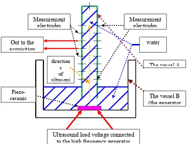
[image:5.595.111.494.243.538.2]In order to study the voltage appeared in the ultrasonic cavitation, we used the appliance drawn in the figure 2. The data obtained, using the acquisition card, at the first degree of power of the ultrasound generator, are represented in the figure 3.
Figure 2. Experimental appliance
Piezo-ceramic
Ultrasound load voltage connected
to the high frequency generator
The vessel B
(the generator
Measurement
electrodes
Measurement
electrodes
water
Out to the
acquisition
The vessel A
direction-12 -9 -6 -3 0 3 6 9 12
[image:6.595.133.477.82.401.2]1 57 113 169 225 281 337 393 449 505 561 617 673 729
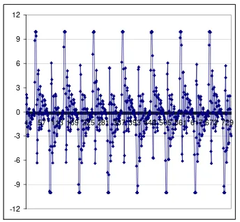
Figure 3. The signal form
It can be seen that there exists a periodicity of the signal and after the study of the given values, the determined period was 105. The study was made only for a period using the Box - Jenkins method.
The model proposed is an ARIMA(2, 0, 0), without a constant term:
,
3
n
,
n
,
V
.
V
.
V
n=
1
5636298
n−1−
0
8913194
n−2+
ε
n∈
N
≥
(7)where
ε
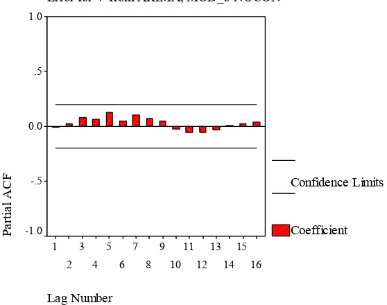
nis the residual, which is a white noise.Error for V from ARIMA, MOD_3 NOCON Lag Number 16 15 14 13 12 11 10 9 8 7 6 5 4 3 2 1 A C F 1.0 .5 0.0 -.5 -1.0 Confidence Limits Coefficient
Figure 4. The autocorrelation function for the residual in the model (7) Error for V from ARIMA, MOD_3 NOCON
[image:7.595.170.449.384.604.2]The values of the Box –Ljung statistics are in the interval
[
0.008,6.234]
, so they are less thanℵ2(100). The probabilities of the acceptance of the white noise hypothesis for the residuals are big, so the residuals form a white noise and the model is well selected.3. CONCLUSIONS
The ultrasonic treatment applied on some material produces them erosion. Also, the cavitation bubbles are electric charged and the existence of that tension was proved using the experimental appliance. The mathematical form of the voltage induced by the cavitation was also determined. In our study (to appear) we saw that this form is different for the different types of liquid.
References
[1] A. Barbulescu, Time series, with applications (in Romanian), Ed. Junimea, Iasi, 2002
[2] J. Bourbonais, Cours et exercices d'econometrie, Dunod, Paris, 1993
[3] C. Gourierous, A. Monfort, Series temporelles et modeles dynamiques, Economica, Paris, 1990
[4] V. Marza, Contributions to the study of the ultrasonic cavitation and of some electrical and chemical phenomena induced by it, PhD. Thesis, Constanta, 2003 (In Romanian)
[5] V. Marza, N. Peride, M. Mititelu, G. Mandrescu, A. Danisor, Electrical phenomena with join acoustic cavitation (to appear)