A MIXED MONTE CARLO AND QUASI-MONTE CARLO SEQUENCE FOR MULTIDIMENSIONAL INTEGRAL
ESTIMATION
Alin V. Ros¸ca
Abstract. In this paper, we propose a method for estimating an s -dimensional integral I. We define a new hybrid sequence that we call the
H-mixed sequence. We obtain a probabilistic bound for the H-discrepancy of this sequence. We define a new estimator for a multidimensional integral using the H-mixed sequence. We prove a central limit theorem for this estimator. We show that by using our estimator, we obtain asymptotically a smaller variance than by using the crude Monte Carlo method. We also compare our method with the Monte Carlo and Quasi-Monte Carlo methods on a numerical example.
2000 Mathematics Subject Classification: 68U20, 65C05, 11K36, 11K45, 11K38.
Keywords and phrases: Monte Carlo integration, Quasi-Monte Carlo inte-gration, H-discrepancy, H-distributed low-discrepancy sequences, H-mixed sequences.
1. Introduction
We consider the problem of estimating integrals of the form
I = Z
[0,1]s
f(x)dH(x), (1)
wheref : [0,1]s
→Ris the function we want to integrate andH :Rs →[0,1] is a distribution function on [0,1]s. In the continuous case, the integralI can be rewritten as
I = Z
[0,1]s
wherehis the density function corresponding to the distribution functionH. In the Monte Carlo (MC) method (see [11]), the integral I is estimated by sums of the form
ˆ
IN = 1
N
N X
k=1
f(xk),
where xk = (x(1)k , . . . , x(s)k ), k ≥ 1, are independent identically distributed random points on [0,1]s, with the common density function h.
In the Quasi-Monte Carlo (QMC) method (see [11]), the integral I is approximated by sums of the form N1 PNk=1f(xk), where (xk)k≥1 is a H -distributed low-discrepancy sequence on [0,1]s.
In [7], [8] and [9], Okten considered integrals of the form
I1 = Z
[0,1]s
f(x)dx,
and proposed a method for estimating the integralI1, using a so-calledmixed sequence on [0,1]s, which combines pseudorandom and low-discrepancy vec-tors. Each element of the s-mixed sequence (xk)k≥1 is obtained by concate-nating two vectors qk and Xk, i.e., xk = (qk, Xk), k ≥ 1, where (qk)k≥1 is a d-dimensional low-discrepancy sequence and Xk, k ≥ 1, are independent uniformly distributed random vectors on [0,1]s−d.
In this paper, we extend the results obtained by Okten to the case when the integral is of the form (1). First, we remember some basic notions and definitions that will be used in this paper. Next, we define a new hybrid sequence that we call theH-mixed sequence and obtain probabilistic bounds for theH-discrepancy of this sequence. Continuing, we define a new estima-tor for the integral I, using ourH-mixed sequence, and prove a central limit theorem for this estimator. In the last paragraph, we consider a numerical example, in which we compare our estimator with the ones obtained by using the MC and QMC methods.
2. A probabilistic bound for the H-discrepancy of the
H-mixed sequence
Definition 1. (H-discrepancy) Consider an s-dimensional continuous distribution on[0,1]s, with distribution function H. Let λ
H be the probability
measure induced by H. Let P = (xk)k≥1 be a sequence of points in [0,1]s.
The H-discrepancy of the first N terms of sequence P is defined as
DN,H(x1, . . . , xN) = sup J⊆[0,1]s
1
NAN(J, P)−λH(J)
,
where the supremum is calculated over all subintervals J = Qsi=1[ai, bi] ⊆ [0,1]s; A
N counts the number of elements of sequence P, falling into the
interval J, i.e.,
AN(J, P) = N X
k=1
1J(xk),
1J is the characteristic function of J. The sequenceP is called H-distributed if DN,H(x1, . . . , xN)→ 0 as N → ∞. The H-distributed sequence P is said
to be a low-discrepancy sequence if
DN,H(x1, . . . , xN) =O (logN)s/N
for all N ≥2.
Definition 2. Consider an s-dimensional continuous distribution on
[0,1]s, with density function h and distribution function H. For a point
u = u(1), . . . , u(s) ∈ [0,1]s, the marginal density functions h
l, l = 1, . . . , s,
are defined by
hl u(l)
= Z
. . .
Z
| {z } [0,1]s−1
h t(1), . . . , t(l−1), u(l), t(l+1), . . . t(s)dt(1). . . dt(l−1)dt(l+1). . . dt(s),
and the marginal distribution functions Hl, l = 1, . . . , s, are defined by
Hl u(l)
= Z u(l)
0
hl(t)dt.
In this paper, we considers-dimensional continuous distributions on [0,1]s, with independent marginals, i.e.,
H(u) = s Y
l=1
This can be expressed, using the marginal density functions, as follows:
h(u) = s Y
l=1
hl(u(l)), ∀u= (u(1), . . . , u(s))∈[0,1]s.
Consider an integer 0< d < s. Using the marginal density functions, we construct the following density functions on [0,1]dand [0,1]s−d, respectively:
hq(u) = d Y
l=1
hl(u(l)), ∀u= (u(1), . . . , u(d))∈[0,1]d,
and
hX(u) = s Y
l=d+1
hl(u(l)), ∀u= (u(d+1), . . . , u(s))∈[0,1]s−d. The corresponding distribution functions are
Hq(u) = Z u(1)
0
. . .
Z u(d) 0
hq t(1), . . . , t(d)
dt(1). . . dt(d), (2) where u= (u(1), . . . , u(d))∈[0,1]d, and
HX(u) =
Z u(d+1) 0
. . .
Z u(s) 0
hX t(d+1), . . . , t(s)
dt(d+1). . . dt(s), (3)
where u= (u(d+1), . . . , u(s))∈[0,1]s−d.
In the following definition, we introduce the new notion of a H-mixed sequence.
Definition 3. (H-mixed sequence) Consider an s-dimensional contin-uous distribution on [0,1]s, with distribution function H and independent
marginals Hl, l = 1, . . . , s. Let Hq and HX be the distribution functions
defined in (2) and (3), respectively. Let (qk)k≥1 be a Hq-distributed
low-discrepancy sequence on [0,1]d, with q k = (q
(1) k , . . . , q
(d)
k ), and Xk, k ≥ 1, be
independent and identically distributed random vectors on [0,1]s−d, with
dis-tribution function HX, where Xk = (X (d+1)
k , . . . , X (s)
k ). A sequence (mk)k≥1,
with the general term given by
is called a H-mixed sequenceon [0,1]s.
Remark 4. For an interval J = Qsl=1[al, bl] ⊆ [0,1]s, we define the subintervals J′ =Qd
l=1[al, bl]⊆[0,1]d and J′′ = Qs
l=d+1[al, bl]⊆[0,1]s−d (i.e.
J =J′ ×J′′).
Let (mk)k≥1 be a H-mixed sequence on [0,1]s, with the general term given by (4). Based on definitions (1) and (3), the H-discrepancy of the set of points (m1, . . . , mN) can be expressed as
DN,H(m1, . . . , mN) = sup J⊆[0,1]s
1 N N X k=1
1J(mk)−λH(J)
= sup
J⊆[0,1]s 1 N N X k=1
1J(mk)− Z
J
dH(u)
= sup
J⊆[0,1]s 1 N N X k=1
1J(mk)− s Y
l=1
[Hl(bl)−Hl(al)] ,
and theHq-discrepancy of the set of points (q1, . . . , qN) is given by
DN,Hq(q1, . . . , qN) = sup J′⊆[0,1]d
1 N N X k=1
1J′(qk)−λHq(J′)
= sup
J′⊆[0,1]d 1 N N X k=1
1J′(qk)−
d Y
l=1
[Hl(bl)−Hl(al)] ,
We consider the random variable 1J(mk) that is taking two values 1 and 0, with the probabilities deduced as follows:
P(1J(mk) = 1) = 1J′(qk)P(Xk∈J′′)
= 1J′(qk)P(Xk(d+1) ∈[ad+1, bd+1], . . . , Xk(s) ∈[as, bs])
= 1J′(qk)P(Xk(d+1) ∈[ad+1, bd+1])·. . .·P(Xk(s)∈[as, bs])
= 1J′(qk)
s Y
l=d+1
where the productQsl=d+1[Hl(bl)−Hl(al)] was denoted byp. Thus,P(1J(mk) = 0) = 1−1J′(qk)p. Hence, the distribution of the random variable 1J(mk) is
1J(mk) :
1 0
1J′(qk)·p 1−1J′(qk)·p
, k ≥1. (5)
Lemma 5. The random variable 1J(mk) has the expectation and the variance given by
E(1J(mk)) = 1J′(qk)p, (6)
V ar(1J(mk)) = 1J′(qk)p(1−p). (7)
Furthermore,
Cov(1J(mi)·1J(mj)) = 0 for i, j ≥1, i6=j. (8)
Proof. We have
E(1J(mk)) = 1·1J′(qk)p+ 0·(1−1J′(qk)·p)
= 1J′(qk)p.
For the variance, we obtain
V ar(1J(mk)) = E(1J(mk)2)−(E(1J(mk)))2 = 1J′(qk)p−1J′(qk)p2
= 1J′(qk)p(1−p).
The distribution of the product 1J(mi)·1J(mj) is
1J(mi)·1J(mj) :
1 0
1J′(qi)1J′(qj)·p2 1−1J′(qi)1J′(qj)·p2
.
Hence, we get
From this, the covariance is
Cov(1J(mi)·1J(mj)) = p2·1J′(qi)1J′(qj)−1J′(qi)p·1J′(qj)p= 0.
Corollary 6. Let 1J(mk) be the random variable defined in (5). Then, we have
E1 N
N X
k=1
1J(mk) = p
N
N X
k=1
1J′(qk), (9)
V ar1 N
N X
k=1
1J(mk) = p(1−p)
N2 N X
k=1
1J′(qk),(10)
V ar1 N
N X
k=1
1J(mk)− s Y
l=1
[Hl(bl)−Hl(al)] ≤ 1
4N[DN,Hq(qk) + 1].(11)
Proof. The first two relations follow immediately from Lemma 5. For the last relation, we have
V ar1 N
N X
k=1
1J(mk)− s Y
l=1
[Hl(bl)−Hl(al)] = p(1−p)
N2 N X
k=1
1J′(qk)
= p(1−p)
N
N X
k=1
1J′(qk)
N
≤ 1
4N[DN,Hq(qk) +
d Y
l=1
[Hl(bl)−Hl(al)]]
≤ 41N[DN,Hq(qk) + 1]. We introduce the following notations:
Z = 1
N
N X
k=1
and
u(J) =Z−λH(J), (13)
where
λH(J) = s Y
l=1
[Hl(bl)−Hl(al)]. (14) We need the following lemma.
Lemma 7. If P(|u(J)|< a)≥p, then P(supJ⊆[0,1]s|u(J)|< a)≥p.
Proof We have
|u(J)|< a, ∀J ⊆[0,1]s. Hence, we get
supJ⊆[0,1]s|u(J)|< a. For the corresponding events, we have the implication
{|u(J)|< a} ⊆ {supJ⊆[0,1]s|u(J)|< a}.
Finally, using a well-known inequality from probability theory, we obtain
p≤P(|u(J)|< a)≤P(supJ⊆[0,1]s|u(J)|< a). Thus, we get the desired inequality
P(supJ⊆[0,1]s|u(J)|< a)≥p.
Our main result, which gives a probabilistic error bound for the H-mixed sequences, is presented in the next theorem.
Theorem 8. If (mk)k≥1 = (qk, Xk)k≥1 is a H-mixed sequence, then
∀ε >0 we have
P(DN,H(mk)≤ε+DN,Hq(qk))≥1− 1
ε2 1 4N
DN,Hq(qk) + 1
. (15)
Proof. We apply the Chebyshev’s Inequality for the random variable
u(J), defined in (13), and obtain
P(|u(J)−E(u(J)|< ε)≥1− V ar(u(J))
which is equivalent to
P(−ε+E(u(J))< u(J)< ε+E(u(J)))≥1− V ar(u(J))
ε2
≥1− 1
ε2 1 4N
DN,Hq(qk) + 1
. (17)
We have the following chain of implications:
−ε+E(u(J))< u(J)< ε+E(u(J))⇒
|u(J)| ≤max(| −ε+E(u(J))|,|ε+E(u(J))|)⇒
|u(J)| ≤supJ⊆[0,1]smax(| −ε+E(u(J))|,|ε+E(u(J))|)⇒
|u(J)| ≤max(ε+DN,Hq(qk), ε+DN,Hq(qk))⇒
|u(J)| ≤ε+DN,Hq(qk). (18)
From relations (17) and (18), we obtain
P(|u(J)| ≤ε+DN,Hq(qk))≥1− 1
ε2 1 4N
DN,Hq(qk) + 1
. (19)
We apply Lemma 7 and get
P(supJ⊆[0,1]s|u(J)| ≤ε+DN,Hq(qk))≥1− 1
ε2 1 4N
DN,Hq(qk) + 1
. (20) Hence, we obtain the inequality that we have to prove:
P(DN,H(mk)≤ε+DN,Hq(qk))≥1− 1
ε2 1 4N
DN,Hq(qk) + 1
. (21)
Remark 9. We know that if (qk)k≥1 is aHq-distributed low-discrepancy sequence on [0,1]d, then
DN,Hq(qk) =O
(logN)d
N
.
Hence
DN,Hq(qk)≤cd
(logN)d
N
If we consider ε= 1 4
√
N in Theorem 8 then, as N → ∞, we have
DN,Hq(qk) + 1
4√N ≤
cd
(logN)d N
+ 1
4√N −→0.
In conclusion, when N → ∞, we have
DN,H(mk)−→0, (22)
with probability
p1 = 1−
DN,Hq(qk) + 1
4√N −→1. (23)
3. An estimator for a multidimensional integral using H-mixed sequences
In order to estimate integrals of the form (1), we introduce the following estimator, which extends the one given by Okten (see [9]).
Definition 10. Let (mk)k≥1 = (qk, Xk)k≥1 be ans-dimensional H-mixed
sequence, introduced by us in Definition 3, with qk = (q (1) k , . . . , q
(d)
k )andXk= (Xk(d+1), . . . , Xk(s)). We define the following estimator for the integral I:
θm = 1
N
N X
k=1
f(mk). (24)
We consider the independent random variables:
Yk =f(mk) =f(q(1)k , . . . , q (d) k , X
(d+1)
k , . . . , X (s)
k ), k ≥1. (25) We denote the expectation of Yk by
E(Yk) =µk, (26)
and the variance of Yk by
We assume that
0< σ2k<∞, (28)
and we denote
0< σ2(N) =σ12+. . .+σN2 <∞. (29)
Remark 11. The estimator θm, defined in relation (24), is a biased estimator of the integral I, its convergence to I being asymptotic
E(θm)→I, as N → ∞.
Proposition 12. We assume that f is bounded on [0,1]s and that the
functions
f1(x(1), . . . , x(d)) = Z
[0,1]s−d
(f(x(1), . . . , x(s)))2 s Y
l=d+1
hl(x(l))dx(d+1)·. . .·dx(s),
f2(x(1), . . . , x(d)) = h Z [0,1]s−d
f(x(1), . . . , x(s)) s Y
l=d+1
hl(x(l))dx(d+1)·. . .·dx(s)i2 are Riemann integrable. Then, we have
σ2 (N)
N −→L, as N −→ ∞,
where
L=
Z
[0,1]s
(f(x(1), . . . , x(s)))2 s Y
l=1
hl(x(l))dx(1). . . dx(s)−
−
Z
[0,1]d h Z
[0,1]s−d
f(x(1), . . . , x(s)) s Y
l=d+1
hl(x(l))dx(d+1)·. . .·dx(s)i2·
·
d Y
l=1
Proof. From the fact that f1 is Riemann integrable, it follows that 1 N N X k=1
f1(qk(1), . . . , qk(d))−→ Z
[0,1]d
f1(x(1), . . . , x(d)) d Y
l=1
hl(x(l))dx(1). . . dx(d) =
= Z
[0,1]d h Z
[0,1]s−d
(f(x(1), . . . , x(s)))2 s Y
l=d+1
hl(x(l))dx(d+1)·. . .·dx(s)i·
·
d Y
l=1
hl(x(l))dx(1). . . dx(d).
As f2 is Riemann integrable, we obtain 1
N
N X
k=1
f2(qk(1), . . . , qk(d))−→ Z
[0,1]d
f2(x(1), . . . , x(d)) d Y
l=1
hl(x(l))dx(1). . . dx(d) =
= Z
[0,1]d h Z
[0,1]s−d
f(x(1), . . . , x(s)) s Y
l=d+1
hl(x(l))dx(d+1)·. . .·dx(s)i2· d
Y
l=1
hl(x(l))dx(1). . . dx(d).
We also know that
V ar(Yk) = σ2k=V ar(f(mk)) =V ar(f(qk(1), . . . , qk(d), Xk(d+1), . . . , Xk(s))) =
Z
[0,1]s−d
(f(qk(1), . . . , qk(d), x(d+1), . . . , x(s)))2 s Y
l=d+1
hl(x(l))dx(d+1)·. . .·dx(s)−
− h Z
[0,1]s−d
f(qk(1), . . . , q(d)k , x(d+1), . . . , x(s)) s Y
l=d+1
hl(x(l))dx(d+1)·. . .·dx(s)i2
= f1(qk(1), . . . , qk(d))−f2(qk(1), . . . , q(d)k ).
Hence, we get
σ2 (N)
N =
σ2
1 +. . .+σN2
N
= PN
k=1f1(q (1) k , . . . , q
(d) k )
N −
PN
k=1f2(qk(1), . . . , q (d) k )
Now, we formulate and prove the main result of this paragraph.
Theorem 13. In the same hypothesis as in Proposition 12 and, in ad-dition, assuming that L6= 0, we have
a)
Y(N) = PN
k=1Yk− PN
k=1µk
σ(N) −→
Y, as N → ∞, (30)
where the random variable Y has the standard normal distribution.
b) If we denote the crude Monte Carlo estimator for the integral (1) by θM C, then
V ar(θm)≤V ar(θM C), (31)
meaning that, by using our estimator, we obtain asymptotically a smaller variance than by using the classical Monte Carlo method.
Proof. a) As f is bounded, it follows that the random variables
Yk=f(mk), k ≥1, (32)
are also bounded.
From the facts that L 6= 0, (σ2
(N))N≥1 is a strictly increasing sequence, and
lim N→∞
σ2 (N)
N =L,
it follows that
lim N→∞σ
2
(N) =∞. (33)
Applying Corollary 5, page 267, from Ciucu [3] for the sequence of indepen-dent non-iindepen-dentically distributed random variables (Yk)k≥1, which are bounded and verify relation (33), it follows that
Y(N)= PN
k=1Yk− PN
k=1µk
σ(N) −→
Y ∈N(0,1) when N → ∞,
b) We know that
V ar(θM C) =
V ar(f(X))
N , (34)
and
V ar(θm) = σ 2 (N)
N2 . (35)
Hence, the relation (31), which we have to prove, is equivalent to
L= σ
2 (N)
N ≤V ar(f(X)). (36)
We apply the Cauchy-Buniakovski inequality [E(X)]2 ≤E(X2) (see [2]) and we obtain
Z
[0,1]d h Z
[0,1]s−d
f(x(1), . . . , x(s)) s Y
l=d+1
hl(x(l))dx(d+1)·. . .·dx(s)i2·
·
d Y
l=1
hl(x(l))dx(1). . . dx(d) ≥
≥ h Z
[0,1]d h Z
[0,1]s−d
f(x(1), . . . , x(s)) s Y
l=d+1
hl(x(l))dx(d+1)·. . .·dx(s)i·
·
d Y
l=1
hl(x(l))dx(1). . . dx(d)i2 =
= h Z [0,1]s
f(x(1), . . . , x(s)) s Y
l=1
hl(x(l))dx(1). . . dx(s)i2
Multiplying with (−1) the above inequality and addingR[0,1]s(f(x
(1), . . . , x(s)))2·
·Qsl=1hl(x(l))dx(1). . . dx(s), we obtain
L≤V ar(f(X)).
4. Numerical example
In this paragraph, we compare our method with the MC and QMC meth-ods on a numerical example. We want to estimate the followings-dimensional integral (s≥1):
I =
Z
[0,1]s
18x(1)x(2)·. . .·x(s−1)(x(s))2ex(1)x(s)
dH(x), (37)
where we consider the distribution function
H(x(1), x(2), . . . , x(s)) = (x(1))2(x(2))2. . .(x(s))2
on [0,1]s. The corresponding density function is h(x(1), x(2), . . . , x(s)) = 2sx(1)x(2). . . x(s). The marginal distribution functions are
H1(x(1)) = (x(1))2, H2(x(2)) = (x(2))2, . . . , Hs(x(s)) = (x(s))2. and their inverses areH−1
i (x(i)) = p
(x(i)), i= 1, . . . , s. The exact value of the integral I is
18(3e−8)2s 3s−2 .
In the following, we compare numerically our estimator θm, with the estimators obtained using the MC and QMC methods. As a measure of comparison, we will use the relative errors produced by these three methods.
The MC estimate is defined as follows:
θM C = 1
N
N X
k=1
f(x(1)k , . . . , x(s)k ), (38)
where xk = (x(1)k , . . . , x (s)
k ), k ≥ 1, are independent identically distributed random points on [0,1]s, with the common distribution function H.
In order to generate such a point xk, we proceed as follows. We first generate a random pointωk = (ωk(1), . . . , ω
(s)
k ), whereω (i)
k is a point uniformly distributed on [0,1], for each i = 1, . . . , s. Then, for each component ωk(i),
i = 1, . . . , s, we apply the inversion method and obtain that H−1 i (ω
with the distribution function H has independent marginals, it follows that
xk = (H1−1(ω (1)
k ), . . . , Hs−1(ω (s)
k )) is a point on [0,1]s, with the distribution function H.
The QMC estimate is defined as follows:
θQM C = 1
N
N X
k=1
f(x(1)k , . . . , x(s)k ), (39)
where (xk)k≥1 = (x(1)k , . . . , x (s)
k )k≥1 is a H-distributed low-discrepancy se-quence on [0,1]s.
In order to generate such a sequence (xk)k≥1, we first consider a low-discrepancy sequence on [0,1]s, ω = (ω(1)
k , . . . , ω (s)
k )k≥1. Then, by applying
the inverses of the marginals on each dimension, we obtain that (xk)k≥1 = (H−1
1 (ω (1)
k ), . . . , Hs−1(ω (s)
k ))k≥1 is a H-distributed low-discrepancy sequence on [0,1]s (see [10]).
During our experiments, we employed as low-discrepancy sequences on [0,1]s the Halton sequences (see [6]).
The estimate proposed by us earlier is:
θm = 1
N
N X
k=1
f(qk(1), . . . , q(d)k , Xk(d+1), . . . , Xk(s)). (40)
where (qk, Xk)k≥1 is an s-dimensionalH-mixed sequence on [0,1]s.
In order to obtain such a H-mixed sequence, we first construct the H q-distributed low-discrepancy sequence (qk)k≥1 on [0,1]d(the distribution func-tion Hq was defined in (2)) and next, the independent and identically dis-tributed random points xk, k≥1 on [0,1]s−d, with the common distribution function HX (the distribution function HX was defined in (3)). Finally, we concatenate qk and xk for each k ≥1.
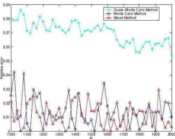
Figure 1: Simulation results fors = 10 and d= 3.
In our tests, we have considered the following dimensions of the integral
I: s = 8, 10, 11, 12, 14, 15. We present the numerical results for a number of 51 samples, having sizes from N = 1000 to N = 2000, with a step size of 20. We have also changed the dimension of the deterministic part of the
H-mixed sequence from d= 3 to d= 8, in order to determine an ”optimal” dimension for the deterministic part of the H-mixed sequence.
The MC and mixed estimates are the mean values obtained in 10 inde-pendent runs, while the QMC estimate is the result of a single run. In our graphs the relative error produced using each of the three methods is plotted against the number of samples N.
Figure 2: Simulation resu1ts fors = 15 and d= 5.
Also, the H-mixed sequences produced a better overall error reduction than the pseudorandom sequences, in both situations we present here. We also re-mark that, in order to achieve these improvements usingH-mixed sequences, the dimension of the deterministic part should be around one third of the problem dimension. Considering a higher dimension of the deterministic component leads us to worse results compared with the MC method. How-ever, the relative errors are still much smaller than the ones produced by using low-discrepancy sequences.
Next, we draw the following conclusions from all the tests we performed, considering the parameters (s, d) presented above:
1. the relative errors for all three estimates are very small, even for small sample sizes,
2. the behavior of the H-mixed sequence is superior to the one of the low-discrepancy sequence, regardless of the dimension of the problem, 3. the performance of the H-mixed sequence is better than the one of the
4. to achieve a good performance of our H-mixed estimator, we observe from our tests that the dimension of the deterministic part should be around one third of the dimension of the problem. However, this is not a general rule and is depending on the test problem or practical situation, where the H-mixed sequence is applied.
In conclusion, by properly chosen the dimension d of the deterministic part in the s-dimensional H-mixed sequence, we can achieve considerable improvements in error reduction, compared with the MC and QMC esti-mates, even for high dimensions and moderate sample sizes.
References
[1] P. Blaga, M. Radulescu, Probability Calculus, Babes-Bolyai University Press, Cluj-Napoca, 1987 (In Romanian).
[2] P. Blaga, Probability Theory and Mathematical Statistics, Vol. II, Babes-Bolyai University Press, Cluj-Napoca, 1994 (In Romanian).
[3] G. Ciucu, C. Tudor, Probabilities and Stochastic Processes, Vol. I, Romanian Academy Press, Bucharest, 1978 (In Romanian).
[4] I. Deak, Random Number Generators and Simulation, Akademiai Ki-ado, Budapest, 1990.
[5] L. Devroye,Non-Uniform Random Variate Generation, Springer-Verlag, New-York, 1986.
[6] J. H. Halton, On the efficiency of certain quasi-random sequences of points in evaluating multidimensional integrals, Numer. Math., 2 (1960), 84-90.
[7] G. Okten,A Probabilistic Result on the Discrepancy of a Hybrid-Monte Carlo Sequence and Applications, Monte Carlo Methods and Applications, Vol. 2, No. 4 (1996), 255-270.
[8] G. Okten, Contributions to the theory of Monte Carlo and Quasi-Monte Carlo Methods, Ph.D. Dissertation, Claremont Graduate School, Cal-ifornia, 1997.
[10] N. Ro¸sca,Generation of Non-Uniform Low-Discrepancy Sequences in the Multidimensional Case, Rev. Anal. Num´er. Th´eor. Approx, Tome 35, No 2 (2006), 207-219.
[11] D. D. Stancu, Gh. Coman, P. Blaga, Numerical Analysis and Ap-proximation Theory, Vol. II, Presa Universitara Clujeana, Cluj-Napoca, 2002 (In Romanian).
Author:
Alin V. Ro¸sca,
Babe¸s-Bolyai University of Cluj Napoca Romania.