THE EXPLANATORY POWER OF MOVING AVERAGE BETA
IN THE JANUARY EFFECT
Krismiati Mukti Ulansari
Consulate General Surabaya - American
ABSTRAK
Beta sebagai pengukur resiko sistematik saham masih menjadi perdebatan hingga saat ini. Beta pasar didasarkan pada asumsi bahwa pasar adalah ‘frictionless’. Asumsi ini tidak relevan dengan kondisi nyata sehingga nilai beta pasar yang dihasilkan akan bias.
Penelitian ini dimaksudkan untuk menguji keunggulan beta moving average (MA) dengan cara menerapkannya di salah satu anomali pasar, yaitu January Effect. Dengan memasukkan unsur ‘friction’ yang ada di pasar ke dalam perhitungan beta, diharapkan beta moving average bisa menjadi pengukur resiko sistematik yang lebih baik.
Hasil studi menunjukkan bahwa ketika diterapkan di January Effect, beta moving average lebih unggul (powerful) daripada beta model pasar karena beta moving average mempunyai nilai adjusted R Square yang signifikan, sedangkan beta model pasar tidak memiliki adjusted R Square yang signifikan. Tetapi studi ini tidak bisa menyimpulkan bahwa beta moving average lebih unggul (powerful) daripada beta model koreksi kesalahan karena nilai adjusted R Square dari beta model koreksi kesalahan negatif. Hasil ini sekaligus menunjukkan bahwa January Effect disebabkan oleh friction yang ada di pasar.
Keywords: moving average beta, error correction model beta, market model beta, market frictions, January Effect.
INTRODUCTION
Since it has been introduced at the first time until recently, CAPM and beta is debatable theoretically and empirically. In the 1990, the debate about whether beta is dead or alive has heated up once again. One school of thought led by Fama and French, writing in the June 1992 issue of the Journal of Finance. Fama and French, launched a forceful attack on the nearly 30 years old CAPM. Their conclusion; beta is the wrong measure of risk. And if beta is not the appropriate predictor of risk, then perhaps risk is not related to returns in the way financial theorists have predicted for two decades (Nichols, 1993). Roll and Ross (1996) demonstrates that beta is dead, or if not
dead is at least fatally ill, because beta fails to explain the behavior of security returns. Contrary with previous thought, the other school of thought led by Kothari, Shanken, and Sloan (1995), Kandel and Stambaugh (1995) shows that beta is alive if annual returns instead of monthly or daily returns are used as input data.
methods: Scholes and Williams, Dimson and Fowler and Rorke. They found that Fowler-Rorke Model with lead-1 and lag-1 is the best model to adjust beta bias in non-synchronous trading activities. Whilst Thanh (2001) found that compared with Fowler and Rorke Model, Error Correction Model actually improve the quality of beta estimates.
Market model beta is derived from CAPM with an assumption that market is frictionless. It is clear that this assumption do not hold in the real world just as it is clear that the frictionless environment does not really exist. Beta is a function of market returns, its estimated value is distorted if returns are contaminated by market frictions. When market frictions, such as transaction cost, information asymmetry, and a host of regulatory restrictions exist, then the arbitrage process is retarded and the explanatory power coefficients are significant, which suggest that
beta is not dead in Fama and French’s time
series analysis. This research implies that the explanatory power of beta is weakened due to observed returns being contaminated by market frictions. It then seems plausible to conjecture that the explanatory power of beta may be reinforced if beta is strengthened to accommodate the market frictions.
Chen et. al. (2000) treat the problem of market frictions by incorporating an optimal lead/lag structure of market returns into the body of their moving average beta.
Researcher is motivated to test other model of beta in Jakarta Stock Exchange because beta is at the heart and soul of a large number of theoretical as well as empirical financial studies, so a clarification about this issue is necessary.
This study will apply moving-average beta model in the Jakarta Stock Exchange. To sharpen the focus, the analyses concentrate on the January effect because this market anomaly is the difficult phenomenon to be explained. That is, the five-factor model of Fama and French (1993) even cannot explain this phenomenon. It is hoped that moving average beta, which accommodates market frictions, has explanatory power in January effect as shown by its significant value of adjusted R square. If moving average beta is capable of explaining the January effect, the preposition that beta is not dead cannot be rejected. More specifically, this study is aimed to answer the following questions: (1) Does January effect exist at the Jakarta Stock Exchange? (2) Does moving average beta have significant explanatory power in the January effect? (3) Is the explanatory of moving average beta superior to the others type of beta (market model or error correction model beta)?
three-factor model are significant. This condition suggest that beta is not dead in Fama
and French’s time series analysis.
Chen et. al., (2000) proposed another approach in treating the problem of market frictions by incorporating an optimal lead/lag structure of market returns into the body of beta itself. The result shows that moving average beta is alive, as its beta coefficient is significant. This study also proves that the explanatory power of moving average beta is superior to OLS beta, Scholes/Williams beta, and Fama and French Sum-beta.
Meanwhile some studies, which try to challenge the hypothesis that security prices are informationally efficient comes from the anomaly literature, which has discovered puzzling patterns in the behavior of asset prices. One such pattern is January seasonal in equity returns, called as January effect.
The phenomenon of abnormal return in January was found by Rozeff and Kinney in 1976 for the first time, but has not been able to explain this phenomenon yet. Numerous theories have been hypothesized to explain the January effect such as the popular tax loss selling and portfolio re-balancing hypothesis. Tax loss selling hypothesis suggests that individuals sell stock losers before year-end to recognize capital losses and reinvest at the turn of the year. Tax loss selling hypothesis is weakened by the finding of Corhay, Hawawini, Michel (1987), and Coutts (1997) who show high January returns also exist in countries where fiscal year-ends are different from the calendar year-ends.
Other studies try to explain January Effect through portfolio re-balancing hypothesis. This hypothesis states that the high returns for risky assets in January are caused by systematic shifts in portfolio holdings of investors, particularly institutional investors, for the purpose of window dressing at the turn of the year. This portfolio re-balancing hypothesis is, in fact, contradicted by Ritter and Chopra (1989) when they demonstrated high January
returns exist not only for losers but also for winners.
Another study concerning about market anomalies is done by Chatterjee and Maniam (1997), who used multivariate regression to test the presence of size effect and January effect. Evidence indicates the presence of significant January effect for small firms.
In Jakarta Stock Exchange, Sindang (1997) tried to study about January Effect in Jakarta Stock Exchange during 1994 - 1997. He found that January effect only exists during in 1996 significant relationship between January effect and firm size in 1995 and 1997.
To verify the existence of January effect in Jakarta Stock Exchange, researcher tries to re-test whether stocks listed in Jakarta Stock Exchange have an excess return in the turn of the year. More specifically, the first hypothesis could be describe as follow:
H1 : There is a difference between portfolio mean return of the five trading days around January and portfolio mean return of the other days for the whole eight years.
To date no one has identified any convincing reason on January effect. Even the five-factor model of Fama and French (1993) does not have any visible explanatory power in the January effect. They suggest that some other fundamental factors deeply rooted in the microstructure of security return may underlie the January effect.
proposition that beta is not dead cannot be rejected. And finally, the proposition that states; a fundamental factor that causes the explanatory power in January Effect.
The study of Chen, et. al. (2000) found that moving average beta does make a significant improvement in explanatory power over and above the Fama and French sum-beta, the Scholes/Williams beta and the OLS beta for explaining the turn-of-the-year effect. In testing the superiority of moving average beta, this study compares the explanatory power of beta or error correction model beta.
METHODOLOGY since the first trading day in January 1991 until the last trading day in December 1998, (2) The company must have an outstanding number of shares for each year since 1991 until 1998.
Data Analysis
To come up with the conclusion, data is analyzed by using analytical step, which
followed Chen, et. al.’s (2000) procedure.
1. For each year ten portfolios that consist of nine firms for each portfolio, are created.
Portfolio are organized based on firm size from small to large, where size is the product of the closing price on the last trading day in December on each year, multiplied by the outstanding number of shares of the company on that day. The smallest size portfolio is denoted Portfolio 1 and the largest is denoted Portfolio 10. 2. Test the January Effect : To investigate the
existence of January Effect, the following steps are applied: where, rjyt is equally-weighted average of stock return i in portfolio j for the trading day t and for the year y. b. Measure daily portfolio return and
market return of the other days (outside the five trading days around January) for the whole period (8 years), which later mentioned as grand sample. c. Compare the mean and standard
d. Test of the Hypothesis
i portfolio j for trading day t j : portfolio 1,....,10
: beta error correction model
5. Compared the result of Cross Sectional test regression model at equation (4) for all types of beta (moving average beta, market model beta, and error correction model beta), in order to investigate the superiority of moving average beta model relative to two other types of beta model.
RESULT
Test the January Effect
January returns are concentrated in small
firms’ returns for the first few trading days
around January.
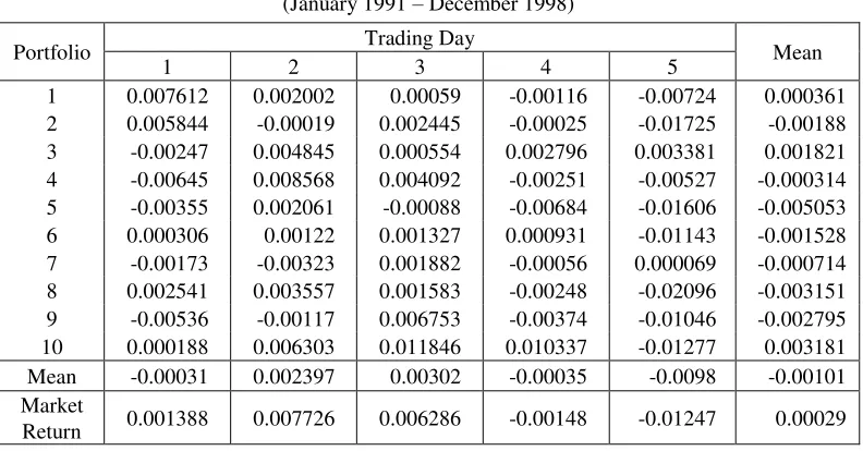
To verify the results of previous studies and to serve as the basis for further analyses, Table 1. reports a summary of the observations for January returns.
Table 1. shows that the average portfolio mean return of the five trading days around January is negative and much lower than the average market return. Since those ten portfolios do not have excess return on January, this evidence indicates that those ten portfolios might not experience January effect. Meanwhile, note that market has positive returns on five trading days around January, which indicates that market as a whole might experience January effect.
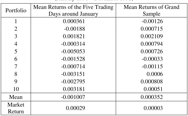
To justify the existence of January effect, the portfolio mean returns of the five trading days around January is compared with the portfolio mean returns of the other days for the whole eight years (grand sample), which consist of 1,955 trading days. Those ten portfolios enjoy January effect if the average portfolio mean return of the five trading days
around January is above the average portfolio mean return of grand sample. The comparative result is reported on the Table 2.
Table 2. reports that those ten portfolios do not experience January effect as the average portfolio mean return of the five trading days around January is much lower than the average portfolio mean return of the other days for the whole eight years (grand sample). Meanwhile the average market return of the five trading days around January is bigger than the average market return of grand sample.
Since those ten portfolios do not have excess returns on the five trading days around January during 1991 – 1998, it is worth to investigate their return behavior at the different period. Based on the consideration that Indonesia has experienced economic crisis since the middle of 1997, which might influence the behavior of some stock at Jakarta Stock Exchange, data in the year after 1996 (1997 and 1998) will be excluded from the sample. It is expected that those ten portfolios have excess returns around January during 1991 – 1996.
Table 1. Mean Returns of the Five Trading Days around January (January 1991 – December 1998)
Portfolio Trading Day Mean
1 2 3 4 5
1 0.007612 0.002002 0.00059 -0.00116 -0.00724 0.000361 2 0.005844 -0.00019 0.002445 -0.00025 -0.01725 -0.00188 3 -0.00247 0.004845 0.000554 0.002796 0.003381 0.001821 4 -0.00645 0.008568 0.004092 -0.00251 -0.00527 -0.000314 5 -0.00355 0.002061 -0.00088 -0.00684 -0.01606 -0.005053 6 0.000306 0.00122 0.001327 0.000931 -0.01143 -0.001528 7 -0.00173 -0.00323 0.001882 -0.00056 0.000069 -0.000714 8 0.002541 0.003557 0.001583 -0.00248 -0.02096 -0.003151 9 -0.00536 -0.00117 0.006753 -0.00374 -0.01046 -0.002795 10 0.000188 0.006303 0.011846 0.010337 -0.01277 0.003181 Mean -0.00031 0.002397 0.00302 -0.00035 -0.0098 -0.00101 Market
Table 2. A Comparison between the Mean Returns of the Five Trading Days around January and the Mean Returns of Grand Sample
(January 1991 – December 1998)
Portfolio Mean Returns of the Five Trading Days around January
Mean Returns of Grand Sample
1 0.000361 -0.00126
2 -0.00188 0.000715
3 0.001821 0.002109
4 -0.000314 0.000794
5 -0.005053 0.000726
6 -0.001528 -0.00033
7 -0.000714 -0.00115
8 -0.003151 0.0006
9 -0.002795 0.000808
10 0.003181 0.00051
Mean -0.001007 0.000352
Market
Return 0.00029 0.00003
Table 3. Mean Returns of the Five-Trading Days Around January (January 1991 – December 1996)
Portfolio Trading Day Mean
1 2 3 4 5
1 0.008092 0.002515 -0.00307 0.000507 -0.00549 0.000511 2 0.011393 -0.00553 0.008221 0.004576 -0.00179 0.003374 3 0.000383 -0.00072 -0.00673 0.004415 0.002661 2.4E-06 4 -0.00175 0.002108 0.00653 0.001157 0.001341 0.001877 5 -0.00368 0.005042 0.002614 -0.00268 -0.0086 -0.00146 6 0.002732 0.004579 0.001794 -0.00032 -0.00263 0.001232 7 0.000347 -0.00127 0.004658 -0.00095 0.008421 0.002243 8 0.008277 0.006504 0.002195 0.001167 -0.00142 0.003346 9 -0.00058 0.000379 0.00654 -0.00229 0.001902 0.00119 10 -0.00061 0.009061 0.013077 0.005125 0.006145 0.00656 Mean 0.002461 0.002267 0.003583 0.001072 0.000055 0.001888 Market
Return 0.000127 0.004405 0.009854 -0.00028 0.002832 0.003388
Table 3 shows that by excluding the period of economic crisis (1997 and 1998), both ten portfolios and market have positive average mean returns on the five trading days around January during 1991 – 1996. But, the result does not indicate that small firms enjoy most
This result does not support several previous studies that indicate the presence of significant January effect for small firm. Previous studies found that the higher returns for the small firm, in comparison to the large
firms are generated in the first few days in January. But this study has conformity with a study, done by Sindang (1997) in Jakarta Stock Exchange, found that there is no relationship between firm size and excess return in January.
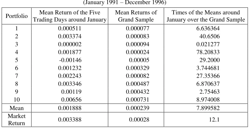
Table 4. A Comparison between the Mean Returns of the Five Trading Days around January the Mean Returns of Grand Sample
(January 1991 – December 1996)
Portfolio Mean Return of the Five Trading Days around January
Mean Returns of Grand Sample
Times of the Means around January over the Grand Sample
1 0.000511 0.000077 6.636364
2 0.003374 0.000083 40.6506
3 0.000002 0.000094 0.021277
4 0.001877 0.000024 78.20833
5 -0.00146 0.00005 29.2000
6 0.001232 0.000329 3.744681
7 0.002243 0.000082 27.35366
8 0.003346 0.000487 6.870637
9 0.00119 0.000432 2.75463
10 0.00656 0.000731 8.974008
Mean 0.001888 0.000239 7.899582
Market
Return 0.003388 0.00028 12.1
To deeply explain the January effect, the portfolio mean returns of the five trading days around January is compared with the portfolio mean returns of the other days for the whole six years (grand sample), which involve 1474 trading days. The comparative results are shown in table 4.
Table 4 shows that the portfolio mean returns of the five trading days around January is, on the average, about 7.89 times larger than the portfolio mean returns of grand sample. Virtually, it can be said that those ten portfolios experience January effect during period 1991 – 1996. Market also has an excess return on the five trading days around January, as its average mean return on the five trading days around January is 12.1 times larger than its on the whole six years.
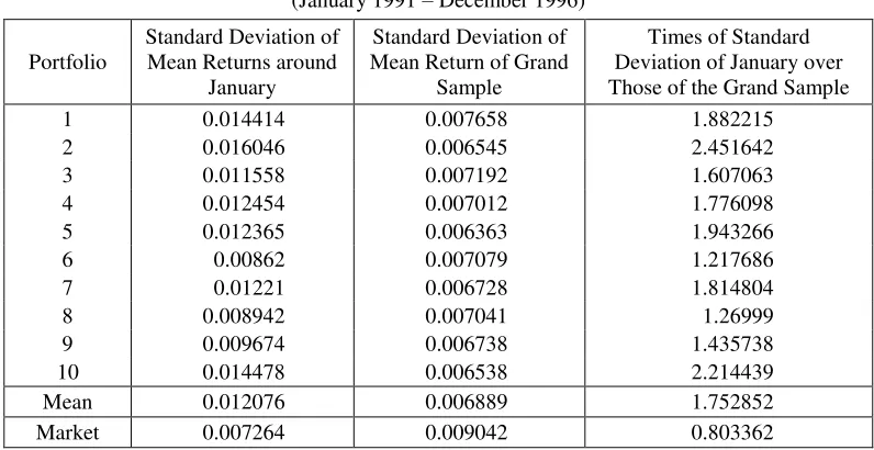
To strengthen the evidence of the January effect, standard deviation of portfolio mean return on the five trading days around January are compared with grand sample at the table 5. below.
Table 5. A Comparison between Standard Deviations of the Mean Returns of the Five Trading Days around January and the Grand Sample
(January 1991 – December 1996)
Portfolio
Standard Deviation of Mean Returns around
January
Standard Deviation of Mean Return of Grand
Sample
Times of Standard Deviation of January over Those of the Grand Sample
1 0.014414 0.007658 1.882215
2 0.016046 0.006545 2.451642
3 0.011558 0.007192 1.607063
4 0.012454 0.007012 1.776098
5 0.012365 0.006363 1.943266
6 0.00862 0.007079 1.217686
7 0.01221 0.006728 1.814804
8 0.008942 0.007041 1.26999
9 0.009674 0.006738 1.435738
10 0.014478 0.006538 2.214439
Mean 0.012076 0.006889 1.752852
Market 0.007264 0.009042 0.803362
To prove the existence of January effect in Jakarta Stock Exchange statistically, the test of Hypothesis 1 is necessary. This hypothesis test uses t-test method to prove that there is a difference between portfolio mean returns of the five trading days around January and portfolio mean returns for the whole six years period. The result of t-test could be seen at the table 6.
The above table shows that the means difference test is significant at the 95% confidence interval. So, we could reject Ho and accepted Ha, which means that there is a difference between portfolio mean returns of the five trading days around January and portfolio mean returns of grand sample. In
other word, the means return of the five trading days around January excess the mean returns of grand sample. So, we can conclude that statistically, there is a January effect in Jakarta Stock Exchange during period 1991 – 1996.
As stated previously, virtually firm size does not influence the excess portfolio return on the five trading days around January. To support this evidence statistically, means difference test between mean returns of the five trading days around January and mean returns of grand sample would also be applied for each portfolio to investigate whether small firm enjoys most of the excess return on January. Table 7 reports the result of t-test for each portfolio.
Table 6. The Result of Means Difference Test between Mean Returns of Five Trading Days around January and Mean Returnof Grand Sample
Mean Difference Std Deviation t-value Sig. (2-tailed) Result Ho Ha 0.001646 0.006495 2.404781 0.018254 Significant Rejected Accepted
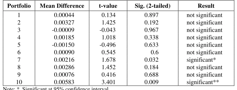
Table 7. The Result of Means Difference Test between Mean Returns of the Five Trading Days around January and MeanReturns of Grand Sample for each Portfolio
Portfolio Mean Difference t-value Sig. (2-tailed) Result
1 0.00044 0.134 0.897 not significant
2 0.00327 1.425 0.192 not significant
3 -0.00009 -0.043 0.967 not significant
4 0.00185 1.018 0.338 not significant
5 -0.00150 -0.496 0.633 not significant
6 0.00090 0.545 0.6 not significant
7 0.00216 1.678 0.032 significant*
8 0.00286 1.452 0.184 not significant
9 0.00076 0.416 0.688 not significant
10 0.00583 3.401 0.009 significant**
Note: * Significant at 95% confidence interval ** Significant at 99% confidence interval
Table 7 shows that mean difference test between mean returns of the five trading days around January and mean returns of grand sample only significant for portfolio 7 and 10. Meanwhile small firms do not have significant mean difference test. This test result strengthens the previous indication that there is no relationship between firm size and excess return around January and January effect does not come from small-cap issues.
Moving Average Beta in The January Effect
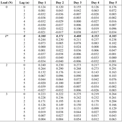
Optimal Lead and Lag Structure
To accommodate the effects of market frictions in the body of the moving average beta is the inclusion of an optimal lead/lag structure of market returns. To identify an
optimal lead/lag structure, MA beta’s equation
and cross section regression test are applied for each trading days around January and for each of the leads from 0 to 3 and for each of the lag from 0 to 7. The values of adjusted R square are summarized at the table 8.
The result shows that there is indeed exists an optimal lead/lag structure, which occurs at the structure of lead-1 and lag-0. The optimal value of adjusted R square is not only the
highest among all lags within the structure of lead-1 but also the highest among 3 leads. The Explanatory Power of Moving Average Beta
To test the second hypothesis, the adjusted R Square values and significance level of moving average beta for the lead-1 and lag-0 are examined at table 9.
Table 9. shows that although the values of adjusted R Square are not relatively high, their values for each trading day are all significant at the 5% significance level. So we could reject Ho and accepted Ha, which means that Moving Average Beta has a significant explanatory power in January Effect.
Moving Average Beta Relative to other types of Beta
Table 8. Adjusted R square for each five trading days around January
Lead (N) Lag (n) Day 1 Day 2 Day 3 Day 4 Day 5
0 0 0.124 0.120 0.155 0.126 0.176
1 0.081 0.043 0.042 0.063 0.072
2 -0.032 -0.036 -0.007 -0.028 0.003
3 -0.038 -0.040 -0.003 -0.034 -0.002
4 -0.032 -0.029 0.000 -0.027 0.016
5 -0.030 -0.037 0.006 -0.030 0.007
6 0.020 0.022 0.106 0.019 0.096
7 -0.021 -0.017 0.038 -0.017 0.034
1* 0 0.388 0.371 0.408 0.353 0.385
1 0.244 0.230 0.211 0.237 0.238
2 0.073 0.085 0.078 0.083 0.102
3 0.000 0.012 0.024 0.008 0.046
4 0.001 0.022 0.036 0.006 0.047
5 -0.037 -0.038 -0.006 -0.032 -0.001
6 -0.035 -0.040 -0.003 -0.033 0.000
7 -0.034 -0.040 -0.006 -0.032 -0.001
2 0 0.240 0.230 0.273 0.217 0.254
1 0.264 0.290 0.268 0.273 0.291
2 0.132 0.176 0.141 0.143 0.163
3 0.067 0.096 0.090 0.069 0.103
4 0.044 0.064 0.072 0.042 0.076
5 -0.020 -0.100 0.007 -0.013 0.013
6 -0.039 -0.040 -0.007 -0.034 -0.002
7 -0.027 -0.032 0.006 -0.026 0.003
3 0 0.223 0.222 0.275 0.219 0.264
1 0.228 0.236 0.242 0.232 0.261
2 0.171 0.195 0.181 0.179 0.204
3 0.126 0.149 0.150 0.131 0.166
4 0.107 0.119 0.131 0.099 0.129
5 0.019 0.038 0.044 0.027 0.050
6 0.007 0.027 0.033 0.017 0.043
7 0.004 0.004 0.054 0.012 0.063
Note : * indicate the optimal value of adjusted R Square
Table 9. Adjusted R Square, and Significance Level for the lead-1 and lag-0
Day 1 Day 2 Day 3 Day 4 Day 5 Mean
Adjusted R Square 0.3880 0.3710 0.4080 0.3530 0.3850 0.3810 Significance Level 0.0000 0.0000 0.0000 0.0000 0.0000 0.0000
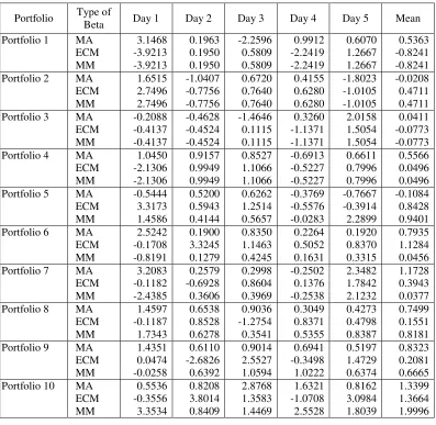
Table 10. The Value of Moving Average Beta Relative to Others Type of Beta
Portfolio Type of
Beta Day 1 Day 2 Day 3 Day 4 Day 5 Mean
Portfolio 1 MA 3.1468 0.1963 -2.2596 0.9912 0.6070 0.5363 ECM -3.9213 0.1950 0.5809 -2.2419 1.2667 -0.8241 MM -3.9213 0.1950 0.5809 -2.2419 1.2667 -0.8241 Portfolio 2 MA 1.6515 -1.0407 0.6720 0.4155 -1.8023 -0.0208 ECM 2.7496 -0.7756 0.7640 0.6280 -1.0105 0.4711 MM 2.7496 -0.7756 0.7640 0.6280 -1.0105 0.4711 Portfolio 3 MA -0.2088 -0.4628 -1.4646 0.3260 2.0158 0.0411 ECM -0.4137 -0.4524 0.1115 -1.1371 1.5054 -0.0773 MM -0.4137 -0.4524 0.1115 -1.1371 1.5054 -0.0773 Portfolio 4 MA 1.0450 0.9157 0.8527 -0.6913 0.6611 0.5566 ECM -2.1306 0.9949 1.1066 -0.5227 0.7996 0.0496 MM -2.1306 0.9949 1.1066 -0.5227 0.7996 0.0496 Portfolio 5 MA -0.5444 0.5200 0.6262 -0.3769 -0.7667 -0.1084 ECM 3.3173 0.5943 1.2514 -0.5576 -0.3914 0.8428 MM 1.4586 0.4144 0.5657 -0.0283 2.2899 0.9401 Portfolio 6 MA 2.5242 0.1900 0.8350 0.2264 0.1920 0.7935 ECM -0.1708 3.3245 1.1463 0.5052 0.8370 1.1284 MM -0.8191 0.1279 0.4245 0.1631 0.3315 0.0456 Portfolio 7 MA 3.2083 0.2579 0.2998 -0.2502 2.3482 1.1728 ECM -0.1182 -0.6928 0.8604 0.1376 1.7842 0.3943 MM -2.4385 0.3606 0.3969 -0.2538 2.1232 0.0377 Portfolio 8 MA 1.4597 0.6538 0.9036 0.3049 0.4273 0.7499 ECM -0.1187 0.8528 -1.2754 0.8371 0.4798 0.1551
MM 1.7343 0.6278 0.3541 0.5355 0.8387 0.8181
Portfolio 9 MA 1.4351 0.6110 0.9014 0.6941 0.5197 0.8323 ECM 0.0474 -2.6826 2.5527 -0.3498 1.4729 0.2081 MM -0.0258 0.6392 1.0594 1.0222 0.6374 0.6665 Portfolio 10 MA 0.5536 0.8208 2.8768 1.6321 0.8162 1.3399 ECM -0.3556 3.8014 1.3583 -1.0708 3.0984 1.3664
MM 3.3534 0.8409 1.4469 2.5528 1.8039 1.9996
The Explanatory Power of MA Beta Relative to the Others Types of Beta
To investigate the explanatory power of moving average beta relative to the other types of beta, Cross-sectional regression test is applied for each type of beta.
From Table 11, first, consider the t-value of beta coefficient. The t-value of a1 (the coefficient of beta) is significant at 5% significance level for moving average beta, but it is not significant for both error correction model and market model beta. Second, note
findings indicate that moving average beta has significant and higher explanatory power in the January effect than market model beta. But the result does not indicate that beta has higher explanatory power than error correction model
beta as its adjusted R Square’s value is
negative. It means that we could reject Ho and accept Ha, states that theexplanatory powerof moving average beta is superior to market model beta.
Table 11. Statistic of the Cross-Sectional Regression Test
Moving Average Error Correction Market Model
Adjusted R Square 0.3810 -0.0222 0.0042
Significant 0.0000 0.6728 0.3796
Coefficient of :
Constant (a0) 0.00033 0.0018 0.0017
Beta (a1) 0.00263 0.0001 0.0006
Dummy (a2) -0.00006 0.0000 0.0000
t-ratio of :
Constant 0.546 2.3528 2.1674
Beta 5.551 0.2946 1.1542
Dummy -0.0154 0.001 -0.015
Sig. Level of :
Constant 0.5518 0.6728 0.0492
Beta 0.0000 0.0306 0.2626
Dummy 0.2826 0.4798 0.4462
Moving average beta is robust and does make a significant improvement over and above market model beta for explaining January effect. The contribution of the moving average beta can be attributed to the improvement in the capability of accommo-dating market frictions. The explanatorypower of moving average beta (as shown by the value of adjusted R square) that accommodates market friction is significant in January effect, while the explanatory power of market model beta that does not accommodate market friction is not significant in the January effect. The test results are consistent with the proposition that a fundamental factor that causes the persistence of January effect is the existence of market frictions.
This test result also gives evidence that beta is seriously ill and its explanatory is weakened if the effects of market frictions are ignored. But beta is still alive and its explanatory power is strengthened if the effects
of market frictions are accommodated and treated.
CONCLUSION
the findings made by previous study that indicated the presence of significant January effect for small firm, the mean returns of the ten portfolios are not virtually monotonically declining as the size of firms become larger. The means difference test also proves that there is no difference in mean return between five trading days around January and grand sample for small firms.
Moving average beta has explanatory power in January effect since its adjusted R Square, which is 0.3810, is significant at 95% confidence interval. As moving average beta, which accommodates the effect of market frictions, has explanatory power in January effect, it seem plausible that a fundamental factor causing January effect comes about from the persistence of market frictions. Moving average beta is robust and does make a significant improvement in explanatory power over and above market model beta. Moving average beta has significant and higher value of adjusted R Square than market model beta. As the market frictions are incorporated into the body of moving average beta, this result indicates that beta is alive or has explanatory power if the effects of market frictions are accommodated and treated. But, beta is seriously ill or has no explanatory power if the effects of market frictions are ignored.
BIBLIOGRAPHY
Chatterjee, A., and Maniam, B., Market Anomalies Revisited, Journal of Applied Business Research, Fall, 1997.
Chen, B.Y., Hsia, C.C., Fuller, C.R., Is Beta Dead or Alive?, Journal of Business Finance and Accounting, April/May, 2000.
Cohen, K.j., Hawawini, G.A., Maier, S.F., Schwartz, R.A., Whitcomb, K.K., Friction in the Trading Process and the Estimation of Systematic Risk, Journal of Financial Economics, August, 1983.
Corhay, A., Hawawini, G.A., and Michel, P, Seasonality in the Risk-return Relationship: Some International Evidence, Journal of Finance, vol. 42, 1987.
Coutts, J.A., Discussion of Microstructure and Seasonality in the UK Equity Market, Journal Of Business Finance and Accounting, Vol 24, 1997.
Fama, E., and French, K., Common Risk Factors in the Returns on Stocks and Bonds, Journal of Financial Economics, February, 1993.
Hartono, J., and Surianto, Bias in Beta Values and its Correction : Empirical Evidence from the Jakarta Stock Exchange, Gajah Mada International Journal of Business, September, 2000.
Nichols, N.A., Efficient? Chaotic, What’s the
New Finance, Harvard Business Review, March-April, 1993.
Sindang, E., Efek Januari (The January Effect) pada Return Saham di Bursa Efek Jakarta periode 1994-1997, Unpublished Internship Report, 1997
Ritter, J.R., and Chopra, N., Portfolio Re-balancing and the Turn-of-the-year Effect, Journal of Finance, 1989.