www.elsevier.com/locate/spa
Phase segregation dynamics for the Blume–Capel model
with Kac interaction
R. Marra
a;∗, M. Mourragui
baDipartimento di Fisica e Unita INFM, Universita di Roma Tor Vergata, Via della Ricerca Scientica,
00133 Roma, Italy
bUPRESA 6085, Universite de Rouen, 76821 Mont Saint Aignan, France
Received 17 May 1999; received in revised form 6 December 1999; accepted 10 December 1999
Abstract
We consider the Glauber and Kawasaki dynamics for the Blume–Capel spin model with weak long-range interaction on the innite lattice: a ferromagneticd-dimensional lattice system with the spin variable taking values in {−1;0;1} and pair Kac potential dJ((|i−j|)); ¿0; i; j∈
Zd. The Kawasaki dynamics conserves the empirical averages of and 2 corresponding to
local magnetization and local concentration. We study the behaviour of the system under the Kawasaki dynamics on the spatial scale −1 and time scale −2. We prove that the empirical averages converge in the limit→0 to the solutions of two coupled equations, which are in the form of the ux gradient for the energy functional. In the case of the Glauber dynamics we still scale the space as −1 but look at nite time and prove in the limit of vanishing the law of large number for the empirical elds. The limiting elds are solutions of two coupled nonlocal equations. Finally, we consider a nongradient dynamics which conserves only the magnetization and get a hydrodynamic equation for it in the diusive limit which is again in the form of the ux gradient for a suitable energy functional. c2000 Elsevier Science B.V. All rights reserved.
Keywords: Interacting particle and spin systems; Kac potential; Hydrodynamic limits; Phase segregation
1. Introduction
We consider particle models which are dynamical versions of lattice gases with Kac potentials. The Kac potentials are functions J(r); r ∈ Rd; ¿0, such that J(r) =
dJ(r), where J is a smooth function of compact support. They have been
intro-duced to describe particle (or spin) systems with weak long-range interaction between two particles (Kac et al., 1963). In the limit → 0 the van der Waals theory of phase transition holds exactly for these models (Lebowitz and Penrose, 1963). Here we propose to consider a Blume–Capel model with Kac interaction that we call Kac– Blume–Capel (KBC) model. The Blume–Capel model is a spin system on the lattice with nearest-neighbour interactions such that the spin variable can assume three val-ues: −1;0;1. It has been introduced originally to study the He3–He4 phase transition
∗Corresponding author.
(Blume, 1966; Capel, 1966). The structure of the phase diagram at low temperature for this model is well understood in terms of the Pirogov–Sinai theory (Bricmont and Slawny, 1989).
The KBC model is dened by the formal Hamiltonian
H() =
1 2
X
i; j∈Zd
J(i−j)((i)−(j))2−h1
X
i∈Zd
(i)−h2
X
i∈∈Zd
2(i); (1.1)
where h1 and h2 are two real parameters. In Section 2 we provide for this model
an analogue of the Lebowitz–Penrose theorem, showing that in the limit → 0 the mean eld theory of the Blume–Capel model (Blume et al., 1971) becomes exact. The equilibrium properties and the phase diagram of the model in the limit → 0 are very interesting. There are two order parameters characterizing the equilibrium Gibbs measure: the magnetizationm, the mean value of the spin, and the concentration, the mean value of the square of the spin. For inverse temperaturenot larger than a critical valuecthere is a unique Gibbs measure which is indeed a Bernoulli measure (as usual
for these mean eld theories), while for temperatures suciently small (and suitable values of the parameters h1 andh2) the Gibbs measure is a superposition of Bernoulli
measures corresponding to dierent values of the couple m; . In particular, there is a point in the phase diagram where there are three extremal equilibrium measures, corresponding to positive, zero and negative magnetization.
We study two Markov processes in the innite volume spin conguration space
generated by self-adjoint operators in L2(; ), where is a Gibbs measure for some
; h1; h2 and nite : the so-called Glauber and Kawasaki dynamics. They can be
de-scribed in words as follows: in the Glauber dynamics each spin at random times ips to a new value or stays unchanged with probabilities depending on the dierence of energy before and after the ip. In the Kawasaki dynamics two neighbouring spins at random times exchange their values, or stay unchanged, with jump rates again depend-ing on the energy dierence. The latter stochastic evolution conserves the dierence and the sum between the number of spins plus and minus (respectively, total mag-netization and total concentration), while the former does not. Moreover, the jump rates depend on the magnetic elds h1; h2 in the Glauber dynamics and do not in the
Kawasaki one. As a consequence, all the Gibbs measures regardless of the values of
h1; h2 are invariant for the Kawasaki dynamics, while for the Glauber dynamics the
only invariant measures are the Gibbs measures with the values ofh1; h2 equal to those
appearing in the jump rates.
We scale the lattice spacing byand look rst at the behaviour of the system under the Glauber dynamics in the limit → 0. We show that the empirical averages of magnetization and concentration converge weakly in probability to the solution of the set of two coupled non-local equations (3.7) and (3.8) (in Section 3).
To get a denite limit in the case of the Kawasaki dynamics we have to scale also the time as −2 (Giacomin et al., 1998). This is a process with two conservation
laws. We prove also in this case a law of large numbers for the empirical averages of and2, respectively, magnetization and concentration. Their limits satisfy the set
functional F Z
drf0(u(r)) +1 2
Z
dr
Z
dr′J(r−r′)[m(r)−m(r′)]2; (1.2)
whereu:= (m; ) and f0(u) is
f0(u) :=−m2++−1
1
2(m+) log(m+) + 1
2(−m) log(−m)
+ (1−) log(1−)−log 2
: (1.3)
Eqs. (3.5) become
@tu= d
X
i=1
X
=1;2
@i
M; @i
F
u
(1.4)
and in vectorial form
@tu=∇ ·
M∇F
u
; (1.5)
whereF=u denotes the functional derivative ofF with respect tou andM is the
2×2 mobility matrix
M =(1−)
+
2−m2
1− m
m
: (1.6)
It is easy to see that F is a Lyapunov functional for (1.5). In fact,
d dtF=−
d
X
i=1 2
X
; =1
Z
dr @i
F
u
M; @i
F
u
: (1.7)
The homogeneous minimizers of the functional F coincide with the minimizers of
f0, which has a unique minimizer but is not convex for large enough. The convex
envelope off0 is the free energyf of the KBC model at= 0 and has some at parts
which single out a regionF (forbiddenregion) inD={(m; ):∈[0;1]; m6}; the domain of denition off0, such that for no value of the chemical potentialsh
1; h2 there
is an extremal state with magnetization and concentration in F. Any Gibbs measure with averages m and in F has to be a linear superposition of the extremal states with (m; )6∈F.
These properties of the energy functional should allow to relate concepts of stable, unstable and metastable phases with the behaviour of the solutions of (1.5).
interface motion and the segregation behaviour (see for recent developments Carlen et al., 1999a,b).
We would notice that the mean eld free energy functional for the Ising model is also not convex for large and, since the rst-order phase transition in the Ising model occurs at zero magnetic eld, has a symmetric double-well structure. In the KBC model instead, the phase transition (in the sense of coexistence of phases) takes place at non-zero h1 and=or h2.
Finally, we have also studied a dierent kind of dynamics, which is in a way intermediate between Glauber and Kawasaki in the fact that it conserves only one quantity, the magnetization. Under this dynamics a bond (i; j) (namely a couple of neighbouring sites i and j) changes its conguration ((i); (j)) or stays unchanged, with probability depending on the energy dierence, to a new conguration (′(i); ′(j))
in such a way that in each site of the bond the spin variable changes by 1 and
(i)+(j)=′(i)+′(j). Hence the magnetization stays constant during the evolution,
while the number of 0’s can change. For example, changes from a bond conguration (−1;1) to a conguration (0;0) or from (0;0) to (−1;1) are possible: a sort of anni-hilation and creation process. The jump rates are chosen to satisfy the detailed balance with respect to the Gibbs measures for the Hamiltonian (1.1) with h2= 1. We derive
under the diusive scaling an equation for m, while on such a long time scale has already relaxed to the equilibrium and its eect can be seen in the mobility appearing in the equation for m. This dynamics is of the so-called non-gradient type (Spohn, 1991) and the proof of the hydrodynamic limit relies on the non-gradient method (Varadhan, 1994).
In Section 2 we describe the equilibrium properties of the KBC model and prove the limit→0 for the innite volume free energy and pressure. In Section 3 we introduce the Glauber and Kawasaki dynamics and state the main theorems, whose proofs are contained in Sections 4 and 5. In Section 6 we prove the hydrodynamic limit for the non-gradient dynamics.
The proof of the hydrodynamic limit for the Kawasaki dynamics is based on the method of Guo et al. (1998). This method has been extended to innite volume by Fritz (1990), by using a bound uniform in the volume for the entropy production. In the paper by Yau (1994) a dierent proof of the uniform entropy production bound has been given for Ginzburg–Landau models and in Landim and Mourragui (1997) this approach has been used to prove hydrodynamic limit for a class of zero range models. We follow the latter approach and prove a uniform bound for the entropy production, which is the time derivative of the entropy. Here we consider not the entropy but the relative entropy of the density of the process with respect to the Bernoulli measure
h1; h2 parametrized by the chemical potentials, which is not invariant for the process. Nevertheless, the bound of this production of entropy will be enough for the GPV method to work. In fact, it is easy to show that the Kawasaki dynamics (thought of as a lattice gas dynamics) is a weak perturbation (and reduces at= 0) of the following generalized symmetric exclusion process (GSEP): each particle on the lattice jumps at random times to a nearest-neighbour site x if and only if there is at most one particle in x. Hence, the state of the system on times −2 will be very close to the invariant
uniform bound for this entropy production will be sucient to prove the hydrodynamic limit. The proof in the case of the Glauber dynamics is simpler: martingales methods are enough. In both cases it has been necessary to prove uniqueness theorems for the weak solutions of the limiting equations.
The non-gradient dynamics studied in Section 6 when formulated in the language of lattice gases is a weak perturbation of a non-gradient generalized simple exclusion process introduced in Kipnis et al. (1994). The diusion coecient for this process is not a constant, like in the symmetric exclusion process considered before, but a function of the density as a consequence of the non-gradient character of the dynamics. We work in this case in a torus, the extension to innite volume being more involved because of the non-gradient nature of the problem. The proof is based again on the method of Guo et al. (1988) and on the non-gradient techniques of Varadhan (1994), that have to be adapted to deal with the perturbation. Also in this case, we will use as reference measure the Bernoulli measure, parametrized this time only by the magnetic eld, which is not invariant for the dynamics. As a consequence, since the dynamics is non-gradient, in the limiting equation there is a new term related to the solution of the non-gradient problem for the unperturbed process. The presence of this term is crucial to recognize that the limiting equation is in the form of the gradient ux for a free energy functional. This is a general fact for non-gradient dynamics weakly perturbed by a Kac potential (see Giacomin et al., 2000). The limiting equation is
@tm=∇ ·
∇G m
with the energy functional G(m(r)) of the form Z
dr g0(m(r)) +1 2
Z
dr
Z
dr′J(r−r′)[m(r)−m(r′)]2; (1.8)
where
g0(m) :=−m2−1[12(m+(m)) log(m+(m)) +12((m)−m) log((m)−m)
+ (1−(m)) log(1−(m))−(m) log 2] (1.9)
and (m) =h2ih1;0 with h1 determined as a function of m via m(h1) =hih1;0. The mobility is given by the Einstein relation =D(m)(m), with being the susceptivity and D the diusion coecient, which is given by the Green–Kubo formula (Kipnis et al., 1994). Note that g0(m) coincides with the functional f0 in (1.3), associated to
the Hamiltonian (1.1) forh2= 1, when evaluated in (m; (m)). This is due to the fact
that is a fast variable under this dynamics and in the diusive limit it relaxes to its equilibrium value h2i
h1;0.
2. The Kac–Blume–Capel model
The Blume–Capel model is a model of spins with values 0;±1 with nearest neigh-bours interactions, originally introduced to study the helium phase transition. Here we will introduce Kac–Blume–Capel (KBC) model which is a model of spins taking val-ues in {−1;0;1} on a d-dimensional lattice Zd and interacting by means of a Kac
potential.
A Kac potential is a function J(r); ¿0, such that
J(r) =dJ(r) for allr∈Rd;
whereJ ∈C2(Rd) is a non-negative function supported in the unit ball, with R
RdJ(r)
= 1 and J(r) =J(−r) for all r∈R.
The spin variable in the sitei∈Zd is denoted by(i) and the innite volume phase
space by {−1;0;1}Zd
. A conguration is a function :Zd → {−1;0;+1}, that is an
element of ={−1;0;+1}Zd
. For any ⊂Zd, denote by the restriction to of
the conguration ; ={(i); i∈}.
The Gibbs measure, with potential J(r) and chemical potentials h1; h2 at inverse
temperature ¿0, in a nite volume and boundary condition is the probability measure ; ; on :
; ; () = 1
Z; ; exp (−H(|));
where Z; ; is the normalization constant and H() is the formal Hamiltonian in a
nite subset of Zd, for the conguration
H() =
1 2
X
i; j∈ i6=j
J(i−j) ((i)−(j))2−h1
X
i∈
(i)−h2
X
i∈
2(i); (2.1)
The innite volume Gibbs measure ; is a probability measure on that can be
constructed by some suitable limiting procedure.
The characteristics of models with Kac potentials is that the range of the interaction is −1 and the strength is d, while the total interaction with all the other spins stays
nite independently of . Hence, Kac potential interactions are useful to study the so-called mean eld limit →0. The innite volume free energy for the Kac Ising model has been computed in the limit → 0 by Lebowitz and Penrose (1963), and the result agrees with (and gives rigorous support to) the van der Waals theory. The analogous result for the KBC model is
Theorem 2.1 (Lebowitz–Penrose limit). Let p(; h1; h2) be the pressure in the
ther-modynamic limit at ¿0. Then
lim
→0p(; h1; h2) =(m;:|msup|6;61)[m
2−+−1s(m; ) +h
1m+h2]; (2.2)
s(m; ) =1
2(m+) log(m+)− 1
2(−m) log(−m)
−(1−) log(1−) +log 2: (2.3)
The free energy f(; m; ) is dened as the Legendre transform of the pressure as
f(; m; ) = sup
(h1; h2)
[h1m+h2−p(; h1; h−2)] = CE[−m2+−−1s(m; )];
(2.4)
where CE denotes the convex envelope. The complementary result in the canonical ensemble is
Theorem 2.2. Dene the free energy f(; m; ) at ¿0 as follows: Consider the partition function in the canonical ensemble
Z(N−; N0) =
X
∈
exp (−H()); (2.5)
where is the set of congurations {} ∈ such that the number of spins = 1 is xed to be N− and the number of spins = 0 is N0. Let N be the total number
of spins in a nite volume and put
m= 1
N
N
X
i=1
(i) = 1
N[N−2N
−N0];
= 1
N
N
X
i=1
((i))2= 1
N[N−N
0]: (2.6)
The free energy at ¿0 in the thermodynamic limit is dened as
f(; m; ) := lim ; N−; N0→∞N
−1logZ
(N−; N0);
where the limit is taken in such a way that (2.6) holds. Then
lim
→0f(; m; ) = CE[−m 2+
−−1s(m; )]: (2.7)
The proof of this theorem is similar to the one of the Lebowitz–Penrose theorem (Lebowitz and Penrose, 1963), (see also De Masi and Presutti (1991)) and will not be given explicitly here. We only remark that the proof of Lebowitz and Penrose (1963) is based on a block spin renormalization procedure and the main point in the proof is writing the renormalized Hamiltonian for the block spins (whose expression will depend on the form of the interaction). Since the interaction term in the KBC model is a two-body interaction like in the Ising model, this part of the proof goes through in almost the same way. Obviously, the entropy will depend on the values of the spin and is in fact dierent from the one computed in Lebowitz and Penrose (1963).
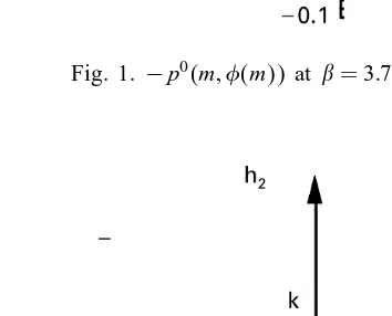
The phase structure of the model at=0 is very rich. To discuss the phase transition we can for example examine the function p0 :=m2−+−1s(m; ) +h
Fig. 1.−p0(m; (m)) at= 3:76; h
1= 0; h2= 0:06.
Fig. 2. Phase diagram at/c.
determining the pressure in (2.2). The extremals of the functionp0 are determined by
the equations
m=tanh(2m+h1);
= exp{(h2−1)}(1−) cosh(2m+h1): (2.8)
These equations can be solved numerically. For6c=12 there is only one solution, while for ¿cthe equations admit more than one solution and the function can have more than one maximum for suitable values ofh1 andh2. For in the interval [12;32]
there is in the plane ; h2 a line of second-order phase transition, which changes to
rst order (made of triple points) at= c andh2= 1 +34ln 2. The point=32; h1= 0;
h2= 1 +43ln 2 is called tricritical point. We refer for details to the paper (Blume et al.,
1971). In Fig. 1 there is the graph of −p0 as a function of m (by means of (2.8)) at a three-phase coexistence point.
The phase diagram in the planeh1; h2, forlarge is shown in Fig. 2. There are three
Fig. 3.f0(m; ) at= 2.
positive (negative) and zero magnetization and along the line h1= 0; h2¿ k there is
coexistence of phases with positive and negative magnetization. Finally, we note that the function
f0:=−m2+−−1s(m; )
is not convex for ¿1
2. In fact
Hess (f0) = 2(m
2−) + 1
(2(1−)(2−m2)): (2.9)
The Hessian is negative in the region−m2¿(2)−1. Hencef, the free energy at
= 0 dened in (2.4) as the convex envelope off0, has some at parts for ¿1 2,
cor-responding to regions in D={m; :∈[0;1]; m6} such that the vectorial function
h(m; ); h:= (h1; h2) cannot be inverted. We call this region inDas a forbidden region
and denote it byF. A point ( m;)∈F has the property that the equationsm(h1; h2) =
m; (h1; h2) = cannot be solved for (h1; h2) (Fig. 3).
Remark. This model can also be looked at as a lattice gas of two species of particles such that in each site of the lattice there is at most one particle for each species. A way of realizing the correspondence is for example the following. Callb(i)=1;0; r(i)=1;0
the occupation number in the siteiof the particles of colours blue and red, respectively. Then, the relation (i) =b(i)−r(i) determines a lattice gas of blue and red particles
with repulsive interaction between particles of the same colour and attractive interaction between particles of dierent colours. Under this correspondence a conguration of particles with two particles in a site i is identical to a conguration with no particles in i.
3. Glauber and Kawasaki dynamics
We consider two kinds of dynamics for the spin system introduced in the previous section: the Glauber and Kawasaki dynamics, the latter conserving both magnetization and concentration.
For (i; j)∈ Zd×Zd; k ∈Zd; ∈ and any cylinder function F:→R, dene
(∇i; jF)(); (∇+kF)() and (∇ −
kF)() by
(∇i; jF)() =F(i; j)−F();
(∇±kF)() =F(±; k)−F();
wherei; j is the conguration obtained from by interchanging the values ati andj:
(i; j) (l) =
(l) if l6=i; j; (j) if l=i; (i) if l=j;
and ±; k is dened as
(±; k) (l) =
(l) if l6=k; (k)±1 mod 3 if l=k:
The Kawasaki dynamics with parameter ¿0 is the unique Markov process on , whose pregenerator LK; acts on the cylinder functions as
(LK;
f)() =
X
i; j∈Zd
|i−j|=1
CK; (i; j;)[(∇i; jf)()]:
Here and in the following |:| stands for the max norm of Rd. For (i; j)∈Zd×Zd and
∈, the rate CK; (i; j;) is given by
CK; (i; j;) ={(∇i; jH())}:
Here:R→R+is a continuously dierentiable function in a neighbourhood of 0, such
that (0) = 1 and satises the detailed balance condition (cf. Giacomin and Lebowitz, 1997; Giacomin et al., 1998)
(E) = exp(−E)(−E): (3.1)
The generator of the Glauber evolution is given by
(LG;
f)() =
X
i∈Zd
CG;±(i;)[(∇±i f)()];
where the rates CG;±
(i;) are dened as
CG;±(i;) =1 2
1
1 + exp ((∇±i H))
corresponding to the choice (E) =12[1 + expE]−1.
Notice that the quantities (∇i; jH) and (∇±i H) are well dened since they involve
In the case of Kawasaki dynamics, if= 0, the evolution reduces to a simple known process. In the setting of the lattice gas with one species of particles this dynamics is a generalized simple exclusion process GSEP (Kipnis and Landim, 1999) with rate one, and we shall denote its pregenerator simply by L0. It diers from the usual SEP
for the exclusion rule involved: in each point are allowed at most two particles. We shall see in Section 3 that the dynamics with ¿0 is a weak perturbation of this simple exclusion. As explained in the remark in Section 3, the Kawasaki dynamics can also be interpreted as the motion of two species of particles, moving as a symmetric simple exclusion process with rate one, with the exclusion rule b+r61, such that
also jumps exchanging colours between neighbour sites are allowed. If such jumps are forbidden the system becomes a non-gradient system and the diusion coecient in this case is dierent from one (Quastel, 1992).
Since the Kawasaki dynamics conserves magnetization and concentration the invari-ant measures will be Gibbs measures parametrized by two chemical potentials. It is useful to introduce the invariant measures for the exclusion process GSEP, which are Bernoulli measures depending on two parameters. For each positive integer n, de-note by n⊂Zd the sublattice of size (2n+ 1)d; n={−n; : : : ; n}d. For A= (a; b)∈
[−1;1]×[0;1], we dene A as the product measure on with chemical potential A
such that, for all positive integers n, the restriction A; n of A ton is given by
d A; n=ZA; n−1exp
(
aX
i∈n
(i) +bX
i∈n
2(i)
)
;
where ZA; n is the normalization constant. For (a; b)∈[−1;1]×[0;1] let m=m(a; b)
(resp. =(a; b)) be the expectation of(0) (resp. 2(0)) under
A; n:
m(a; b) =EA; n((0));
(a; b) =EA; n(2(0)):
Observe that the function dened on ]−1;1[×]0;1[ by (a; b)=(m; ) is a bijection from ]−1;1[×]0;1[ toI={(m; ): 0¡ ¡1;−1¡ m ¡ }. For everyP=(m; )∈I, we denote by P; n the product measure such that
m=EP; n[(0)];
=EP; n[2(0)]: (3.2)
We take −1, the range of the interaction, as macroscopic space unit and consider
the limit → 0. We want to establish for both Kawasaki and Glauber dynamics a law of large numbers for the empirical elds corresponding to magnetization and concentration.
In the Glauber case we look at the behaviour of the elds for nite time, while in the Kawasaki case the relevant time scale is −2. Fix a sequence of probability
measures ()
following sense:
for every continuous function U; V:Rd→Rwith compact support, and every ¿0.
Denote byP(K);
ferentiable functions with compact support.
The main result of this section is the following theorem.
Theorem 3.1. Under (3:3); for any ¿0; t¿0 and U; V∈C2
K(Rd) the following holds:
(i) Kawasaki dynamics:
lim
where ∗ denotes the convolution on the spatial variable. (ii) Glauber dynamics:
where (m(G); (G)) is the unique weak solution of
and ∗ denotes the convolution.
The limiting equations for the Kawasaki dynamics can be rewritten in a nice form as a gradient ux associated with the local mean eld free energy functional. Put
u:= (m; ). Dene the free energy functional as
and the mobility matrix as
M =−[Hess(s)]−1=(1−)
Then Eqs. (3.5) become
@tu=∇
with
f0(u) :=−m2+−−1s(u);
we see thatFreduces for homogeneous proles of magnetization and concentration to
the non-convex free energyf0 of the KBC model, so that the stationary homogeneous solutions of Eqs. (3.5) coincide with the solutions of (2.8). Moreover,Fis a Lyapunov
functional for the evolution, namely it is decreasing in time along the solutions of Eqs. (3.5). This follows from (1.7) and the positivity of the matrix M.
On the contrary, in the Glauber case the limiting equations (3.7) – (3.8) are rather messy. It is not even known if the energy functional is a Lyapunov functional: we have only numerical evidence.
The region D in the plane (m; ), such that D={m; : 0661;|m|6;} can be partitioned for any xed¿c in three parts:
(a) the unstable regionU={(m; )∈F:−m2¿(2)−1}, where F is the forbidden
region dened after (2.9),
(b) the metastable region M ={(m; )∈F:−m2¡(2)−1},
(c) the stable region D−(U∪M).
The segregation phenomena may appear by choosing an initial datum corresponding to total magnetization and concentration in the unstable region. One expects that a stationary solution of Eqs. (3.5) with this initial condition be unstable.
4. Dirichlet form estimates for Kawasaki dynamics
The proof of Theorem 3.1 is based on a priori estimates uniform in the volume for the entropy and the Dirichlet form, which are given in this section. For each positive integer n and a measure on n={−1;0;1}n, we denote by n the marginal of
on n,
n() ={:(i) =(i) for |i|6n} for each ∈n:
For a chemical potential P, and a positive integer n, we denote by sn(n|P; n) the
relative entropy of n with respect to P; n
sn(n|P; n) = sup U∈Cb(n)
Z
U() dn()−log
Z
eU()dP; n()
:
In this formula Cb(n) stands for the space of all functions on n. Since the measure
P; n gives a positive probability to each conguration, all the measures on n are
absolutely continuous with respect to P; n and we have an explicit formula for the
entropy:
sn(n|P; n) =
Z
wherefn is the probability density ofn with respect toP; n. Notice that by the entropy
convexity and since supsupi|(i)| is nite, we have
sn(n|P; n)6C0nd (4.1)
for some constant C0 that depends on P (cf. Kipnis and Landim, 1999).
Dene the Dirichlet form Dn(n|P; n) of the measure n with respect toP; n
associ-ated to the exclusion process by
Dn(n|P; n) =−
Z p
fn()(L0n
p
fn)() dP; n()
= X
i; j∈n |i−j|=1
Ii; j(fn);
whereIi; j(:) is given by
Ii; j(fn) =−
Z p
fn()(L0i; j
p
fn)() dP; n()
and L0
n is the restriction of the process to the box n
L0
n=
X
i; j∈n |i−j|=1
L0
i; j:
Here for a bond (i; j)∈Zd×Zd; L0
i; j stands for the piece of generator associated to
the exchange of spins between sites i andj for the exclusion process.
Dene the entropy S(|P) and the Dirichlet form D(|P) of a measure on
with respect to P as
S(|P) =X n¿1
sn(n|P; n)e−n;
D(| P) =
X
n¿1
Dn(n|P; n)e−n:
Notice that by (4.1), there exists a positive constant C depending on P such that for any probability measure on
S(|P)6C−d: (4.2)
Through this section we consider Kawasaki dynamics with xed parameter ¿0 and with xed scaling parameter −1. We shall denote by (SK;
(t))t¿0 the semigroup
associated to the generator−2LK; (that is, the semigroup of Kawasaki dynamics with
parameter , accelerated by −2). For a measure on we shall denote by K; (t)
the time evolution of the measure under the semigroup SK; :K; (t) =SK; (t).
When=0, the process reduces to the generalized simple exclusion process (Lemma 4.1), and in particular the product measures are invariant for the generatorLK;0
. In this
the exclusion one (Lemma 4.1 below) and adapt Fritz’s approach to that case without considering an approximation of the innite volume dynamics. Notice that from (4.2) there is no need for an initial condition on the entropy in Theorem 3.1.
Lemma 4.1. For any i∈Zd; unit vector e∈Zd and ∈
CK; (i; i+e;) = 1−[(i+e)−(i)]d X
‘∈Zd
(e· ∇J) ((i−‘))(‘)
−d+1[(i+e)−(i)]2(e· ∇J)(0) + O(2)
= 1 +O():
Proof. By denition of H, for all i; j∈Zd and ∈
(∇i; jH)() = 2[(i)−(j)]d
X
‘∈Zd
[J(i−‘)−J(j−‘)](‘)
+2[(i)−(j)]2d[J(i−j)−J(0)]: (4.3)
To prove the lemma, it is enough to remark that the conditions imposed onimply that ′(0) =−1
2 (cf. Giacomin and Lebowitz, 1997) and to use Taylor expansion.
We get the following estimate for the Dirichlet form in the innite volume:
Theorem 4.2. There exists a positive nite constant C1 that depends on P; t and
such that Z t
0
D(K; ()|P) d6C12−d:
The strategy of the proof is to introduce a suitable entropy and Dirichlet form in nite volume and bound the corresponding entropy production in terms of the nite volume Dirichlet form times 2 uniformly in the volume (Lemma 4:2). Then, the a
priori bound on the entropy (4.2) allows to get the estimate.
Fix a measure on and a chemical potential P. For every t¿0 and positive integer n, denote by ft
n the probability density of (K; (t))n with respect to P; n. To
simplify the notation, we denote respectively by sn(fnt) and Dn(fnt) the entropy and
the Dirichlet form of (K; (t))
n with respect to P; n. For all positive integers M, let
M be dened by M=N2 +M, where N=<−1= stands for the integer part of
−1. Dene respectively the entropy SM
(:) and the Dirichlet form DM(:) with nite
sum by
SM (
K; (t)| P) =
M X
n=1
sn(fnt)e −n;
DM (
K; (t)
|P) = M X
n=1
Lemma 4.3. There exist positive and nite constants A0 and A1 that depend on P
and such that; for all positive M
@tSM(
K; (t)
|P)6−−2A0DM(
K; (t)
|P) +A1−d: (4.4)
Before proving the lemma we conclude the proof of Theorem 4.2.
Proof of Theorem 4.2. Integrate (4:4) from 0 to t, letM ↑ ∞and use (4.2).
Proof of Lemma 4.3. We drop the indices in LK; and denote the generator simply
by L. For all positive integers k denote by Lk the restriction of the generator L to
the box k. For a subset A⊂ of Zd, and a function h in L1(P; ), let hhiA be the
function on{−1;0;1}\A obtained by integrating hover the coordinates{(x):x∈A}
with respect to P; . When A=n+m+1−n, we shall denote this expectation simply
by hhim n.
With this notation, we can verify that ft
n satises the equation
@tfnt=−2hL∗n+1fnt+N+1inn+N; (4.5)
where for a positive integerk;L∗
k represents the adjoint operator of Lk inL2(P; k). By
relation (4.5) and the explicit formula for the entropy we have that
@tsn(fnt) = −2
Z
fnt+N+1Lnlog(ft
n) dP; n+N+1
+−2
Z
fnt+N+1(@Ln+1)log(fnt) dP; n+N+1
:=1n+2n: (4.6)
The rst term 1n on the right-hand side of the last inequality corresponds to the exchanges in the interior of n, while the second term 2n is associated to exchanges
at the boundary
(@Ln+1)(f) =
X
i∈n; j6∈n |i−j|=1
CK; (i; j;)[(∇i; jf)()]:
The proof is divided into three steps. In the rst two steps we estimate 1
n and 2n
and in the third one we prove (4:4).
Step1 (bound of1
n). Fix a bond (i; j)∈n×n such that|i−j|= 1, denote byLi; j
the one bond generator corresponding to the exchange of spins between i and j and let Fni; j() be the function dened by Fni; j() =h(CK; (i; j;·)=fnt())fnt+N+1(·)inn+N.
We have
−2
Z
fnt+N+1Li; jlog(ft
n) dP=−2
Z
Fni; j()fnt()log
ft n(i; j)
ft n()
Using the basic inequality
a(logb−loga)6−(√a−√b)2+ (b−a) (4.7)
for positive a and b, the right-hand side of the last expression is bounded by
−−2
Z
Fni; j()[pft n(i; j)−
p
ft n()]
2
dP+−2
Z
Fni; j()[fnt(i; j)−fnt()] dP:
(4.8)
Observe that for all functions h and positive integers n and m;hhn+m+1in+m
n =hn. In
particular, using Lemma 4.1 we have that
|Fni; j()−1|6B:
With this remark, and since the measureP is invariant for the exclusion process, (4.8)
is bounded above by
−−2(1−B)
Z
[pft n(i; j)−
p
ft
n()]2dP+B−1
Z
|fnt(i; j)−fnt()|dP:
Using the elementary inequality 2ab6A−1a2+Ab2, the second term of the last in-equality is bounded by
A
2
−2I
i; j(fnt) +
B
2A
Z
[pft n(i; j) +
p
ft
n()]2dP6
A
2
−2I
i; j(fnt) + 2
B2
A;
where we used in the last inequality Schwartz inequality and the fact that ft n is the
probability density with respect to P. Choosing A small enough, and taking the sum
over all i; j∈n such that |i−j|= 1, we get
1n6−C0Dn(fnt) +C0′nd (4.9)
for some positive constants C0 andC0′.
Step2 (bound of2
n). Fix a bond (i; j)∈n×cn, such that|i−j|=1 and decompose
Li; j into three terms,
Li; j=L(0;1)
i; j +L
(−1;0)
i; j +L
(−1;1)
i; j ; (4.10)
where for (l; m)∈ {(0;1);(−1;0);(−1;1)}; L(l; m)
i; j is given by
(L(l; m)
i; j g)() =r
(l; m)
i; j ()CK; (i; j;)[g(T j; i
m−l)−g()]
+rj; i(l; m)()CK; (i; j;)[g(Ti; j
m−l)−g()]:
Here for = 1;2; (i; j)∈Zd×Zd and a conguration ; Ti; j is dened byTi; j=
−i+j, and r(i; jl; m)() = 1{(i)=l; (j)=m}. Fork ∈Zd; k is the conguration with
spin 1 at site k and none elsewhere, and addition of two congurations is dened coordinate by coordinate.
The term 2
n in (4.6) can be written as a sum of terms2i; j associated to the bond
(i; j). The decomposition (4.10) induces an analogous decomposition for2
i; j. We study
explicitly only the one corresponding to L(−1;1)
i; j , that we denote by
(−1;1)
i; j . The other
two terms are dealt with in the same way:
(i; j−1;1)=−2
Z
fnt+N+1()L
(−1;1)
Let F1i; j andF2i; j be dened by
F1i; j() = 1{(j)=1}CK; (i; j;)fnt+N+1();
F2i; j() = 1{(j)=1}CK; (i; j;j; i)fnt+N+1( j; i):
By changing variables, (i; j−1;1) can be rewritten as
−2
Z
1{(i)=−1}{hF1i; j()inn+N − hF i; j
2 ()inn+N}log
fnt(+ 2i)
ft n()
dP():
(4.11)
Since we have that (a−b) (logc−logd) is negative for a; b; c and d positive real numbers, unlessa¿bandc¿dora6bandc6d, we may introduce in the last integral the indicator function of the set E1
n ∪En2, where
En1={:hF1i; j()i
nn+N
¿hF2i; j()i
nn+N; f t
n(+ 2i)¿fnt()};
En2={:hF1i; j()in+N n
6hF2i; j()in+N n ; f
t
n(+ 2i)6fnt()}:
We shall consider separately the integral onEn1 andEn2, and we call4 (resp. 5) the
integral on the set E1
n (resp. En2). We consider rst the integral on En1 and rewrite it
as the sum of two other terms
4=−2
Z
1{(i)=−1}{hF1i; j()inn+N − hF i; j
3 ()inn+N}
×log
ft
n(+ 2i)
ft n()
1E1
ndP()
+−2
Z
1{(i)=−1}{hF3i; j()inn+N − hF i; j
2 ()inn+N}
×log
ft
n(+ 2i)
ft n()
1E1
ndP();
whereF3i; j is dened by
F3i; j() = 1{(j)=1}CK; (i; j;j; i)fnt+N+1():
Applying Lemma 4.1, we obtain that the rst line of the last expression is of order
−1. Indeed, observe that we have for all congurations
−2hF1i; j()in+N n − hF
i; j
3 ()inn+N
=−2h1{(j)=1}[CK; (i; j;)−CK; (i; j;i; j)]fnt+N+1()inn+N
6C2−1hfnt+N+1()inn+N =C2 −1ft
n()
for some positive constant C2, and on the set En1, we have that fnt(+ 2i)¿fnt().
probability density with respect to P, the rst term of 4 is bounded by
C2−1
Z
1{(i)=−1}|fnt(+ 2i)−fnt()|dP()6C2′
−1
for some positive constant C2′ that depends on P and . We estimate now the second term of 4. Since on En1 we have fnt(+ 2i)¿fnt(), we may replace the indicator
function on E1
n by the indicator function on the set En3 dened by
En3={:hF3i; j()in+N
is less than or equal to
2−2
In particular, the last integral is bounded above by
−3
which, by Schwartz inequality, is bounded by
where we used the fact that there exists a positive constant C4, such that
CK; (i; j;)6C4, for all congurations .
Finally, the second term of (4.12) is bounded by
4−1
for some positive constantC5 that depends onP. We have changed variables and used
the fact that fnt is a probability density with respect toP.
Collecting the above inequalities, we get the following bound for 4. For any
positive
The term5 will be handled in an analogous way. It can be rewritten as
By the same arguments used to estimate 4, we obtain by exchanging the role of
ft
n() andfnt(+ 2i),
56−1(C2′ +C5)
+C4
−2
nX+2N
m=n+N+1 Z
r(j; i−1;1)(){pft m(i; j)−
p
ft
m()}2dP()
for all positive . Therefore, taking advantage of this last inequality and of (4.13), we get
−2
Z
fnt+N+1()L(−1;1)
i; j log (fnt()) dP
62−1(C2′ +C5)
+C4
−2
nX+2N
m=n+N+1 Z
ri; j(−1;1)(){pft m(j; i)−
p
ft
m()}2dP():
+C4
−2
n+2N X
m=n+N+1 Z
rj; i(−1;1)(){pft m(i; j)−
p
ft
m()}2dP():
To conclude this step, we have just to sum over {(0;1);(−1;0);(−1;1)} and over
{(i; j)∈n×nc:|i−j|= 1}. We obtain
2n66nd−1−1(C2′+C5) +C4
−2
nX+2N
m=n+N
Ii; j(fmt) (4.14)
for any positive .
Step 3 (Proof of (4:4)). From (4.6), (4.9) and (4.14), for all positive n @tsn(t)6−C0Dn(fnt) +C0′nd+ 6nd−1−1(C2′ +C5)
+C4
−2
X
(i; j)∈n×c n
nX+2N
m=n+N+1
Ii; j(fmt):
Multiply both sides of this inequality by e−n, sum over 16n6M
and for large
enough. We get for some positive constantsA0 andA1
@tSM(t)6−A0Dn(fnt) +A1−d
+C4′−2
M X
n=M−2N+1
e−n
N X
m=1
X
(i; j)∈n×c n
Ii; j(fmt+n+N):
To conclude the proof of Lemma 4.3, it remains to observe that the third term on the right-hand side of the last inequality is bounded by Const.−d.
Corollary 4.4. For allK ¿0;
Z t
0
DKN(f
KN) d62C1e
Proof. Fix K ¿0 and ∈ [0; t], since by Schwartz inequality n 7→ Dn(fn) is a
non-decreasing function we have
DKN(f KN)6
1
N N X
m=1
DKN+m(f KN+m)
6eK+1 1
N N X
m=1
DKN+m(f KN+m) e
−(KN+m)
62eK+1D(K; ()|P):
5. Hydrodynamic limits for Kawasaki and Glauber dynamics
In this section we prove Theorem 3.1. Let CK(Rd) denote the space of real
continu-ous functions (with compact support) and denote byM the space of signed measures
on Rd with total variation bounded by 1 equipped with the weak∗ topology induced
by CK(Rd) via h; Ui=R Ud.
Given a conguration (t; :), we dene the empirical measures 1; ((t; :)) =1; t ,
and2; ((t; :)) =2; t by
(1t; ; t2; ) =
d X
i∈Zd
(t; i)i; d
X
i∈Zd
((t; i))2i
;
where i is the Dirac mass at the macroscopic site i. We shall denote in the sequel
(t; i) by t(i) and ((t; i))2 by (t; i)2.
5.1. Kawasaki dynamics
First of all, in order to prove (3.4) it is enough to show that, for any positive time
t, any functions U; V ∈CK(Rd) and ¿0,
lim
→0
P(K);
h1t; ; Ui+ht2; ; Vi −
Z
Rd
(m(K)(t; x)U(x)
+(K)(t; x)V(x)) dx
¿
= 0;
where (m(K)(: ; :); (K)(:; :)) is a weak solution of the hydrodynamic equations (3.5). Fix a parameter ¿0 and consider the Kawasaki dynamics atpositive. For a xed time interval [0; T], we denote byP(K) the law of the process (t)t∈[0; T] accelerated by
−2 on the space D([0; T]; ) and by Q(K)
the law of the process (t1; ; t2; )t∈[0; T] on
the space D([0; T];M2) with initial distribution . The law of large numbers for the
empirical measures1t; and2t; follows (Guo et al., 1988) from the weak convergence of the probability measuresQ(K) to a probabilityQ(K) concentrated on the deterministic
trajectory (1(t;dx); 2(t;dx))=(m(K)(t; x) dx; (K)(t; x) dx), where (m(K)(: ; :); (K)(: ; :))
Lemma 5.1 (Tightness). The sequence(Q(K) )is a tight family and all its limit points
Q∗ are such that
Q∗{(1; 2): (1(t;dx); 2(t;dx)) = (1(t; x) dx; 2(t; x) dx)}= 1;
Q∗{(1; 2): −161(t; x)61; 062(t; x)61}= 1:
The proof of Lemma 5.1 is very simple since supsupi|(i)|¡∞ and therefore is omitted.
Lemma 5.2. All limit points Q∗ of the sequence (Q(K) ) are concentrated on weak solutions of Eq. (3:5).
Finally, the law of large numbers follows from the uniqueness of the weak solution of Eqs. (3.5), whose proof is given in Lemma 5.4 below.
Proof of Lemma 5.2. Denote by C1;2
K ([0; T]×Rd) the space of compact support
func-tions V: [0; T]×Rd → R, twice continuously dierentiable on space with
continu-ous derivative in time. Fix a function U= (U1; U2) such that U1(t; x) =Ut1(x) and
U2(t; x) =U2
t(x) are in C
1;2
K ([0; T]×Rd), and consider the martingaleMtU dened by
MtU=
2
X
n=1
hn; t ; Utni − h n;
0 ; U0ni −
Z t
0
(@s+−2LK; )hn; s ; Usnids
with the quadratic variationNU
t given by
NU
t = (MtU)2−
Z t
0
(
−2LK;
2
X
n=1
hn; s ; Usni !2
−2
2
X
n=1
hn; s ; Usni !
−2LK;
2
X
n=1
hn; s ; Usni !)
ds:
Denote by {e1; : : : ; ed} the orthonormal basis of Rd, and observe that for all i ∈Zd,
∈ and k= 1; : : : ; d we have CK; (i+ek; i; ) =ekC K;
(i; i−ek; ), where ek
is the space shift by ek acting on . Hence, a spatial summation by parts permits to
rewrite the integral term of MtU as
2
X
n=1
Z t
0 h
n; s ; @sUsnids
−
2
X
n=1
Z t
0
d−1X
i∈Zd d
X
k=1
CK; (i+ek; i;s)[s(i+ek)n−s(i)n](@kU n s)(i) ds:
Here @k represents the discrete derivative in thekth direction:
(@kV)(i) =−1[V((i+ek))−V(i)]:
Notice that the conditions imposed on imply that ′(0) =−1=2 (cf. Giacomin
parts, we may rewrite the second term of the last integral as
where o(1) is a random variable that converges to 0 with and ∗ stands for the
convolution in the spatial variable. For n= 1;2, the functions gn are dened by
gn() = [(ek)−(0)][(ek)n−(0)n]:
This time, however, it is not the density elds themselves that appear in the second term of the last expression but another local function of the conguration. Following the methods of Guo et al. (1988), the main step in proving the hydrodynamic equations is to replace this local function by another function of the density elds in order to close the equations. For a cylinder function , we denote its expectation with respect to the measure (m; )=P dened in (3.2) by ˜(m; ):
˜(m; ) =Z () dP()
and for a positive integer ‘ and i∈Zd, denote the empirical mean densities on a box
of size (2‘+ 1)d centered at i by (A1; ‘)(i) and (A2; ‘)(i):
Since the support of the function V is compact, by Corollary 4.4 the proof of this lemma is very similar to the one usually used in nite volume. Nevertheless, we shall give a sketch of its proof at the end of this subsection.
can be written as
where@k and@2k represent the rst and the second derivatives in thekth direction, and
o; (1) is a random variable that converges to 0 when →0 and →0.
On the other hand, a simple computation shows that the quadratic variation of the martingale MU
and then it vanishes as goes to 0. By Doob’s inequality, for every ¿0,
lim
Proof of Lemma 5.3. To simplify the notation, for ∈ , denote by VN; () the
convexity and Corollary 4.4, there exists a positive constant C that depends on M;
and P such that the right-hand side of the last inequality is bounded by
for all positive A. It follows that, in order to prove Lemma 5.3 it is enough to show that for each positive A
lim sup
where the supremum is carried over all probability densitiesf with respect to M; N P .
The proof of this limit relies on the usual one and two blocks estimates (cf. Guo et al., 1988; Kipnis et al., 1989) and therefore is omitted.
Lemma 5.4 (Uniqueness). For any T ¿0; Eq. (3:5) has a unique weak solution in the classL∞([0; T])×Rd)×L∞([0; T])×Rd).
Proof. The proof follows the arguments in Giacomin and Lebowitz (1997, 1998) adapted to the innite volume case. For a positive timet ¿0, f∈CK(Rd) and ¿0,
let Hf
t; : [0; t]×Rd→R be dened by Hf
whereht+−s(:) is the heat kernel given by
ht+−s(x) = (2(t+−s))−d=2exp
(
− 1
4(t+−s)
d
X
k=1
(xk)2
)
:
In the appendix it is proven thatHf
t; solves the equation @t= on [0; t]×Rd and
that
d
X
k=1
Z t
0 |h
@kHft; (s; :)i|ds6C1(
√
t+−√)||f||1
6C1
√
t||f||1; (5.1)
whereC1 is a positive constant that depends on dand @k is the rst derivative in the
kth direction.
Let us consider (m; ) and ( ˜m;˜) two weak solutions of (3.5) with the same initial datum. Set m=m−m;˜ =−˜ and W =|m|+||. To keep the notation simple, for (s; x)∈R+×Rd, we shall denote m
s(x) = m(s; x) and s= (s; x). For 16k6d
ands ¿0, let Mk and Fk be dened by
Mk(ms; s) = (s−m2s)(@kJ∗ms);
Fk(ms; s) =ms(1−s)(@kJ∗ms):
Observe that for alls∈[0; t],
Mk(ms; s)−Mk( ˜ms;˜s) = (@kJ∗ms)( ˜s−m˜2s) + (@kJ∗ms)[ s−ms(ms+ ˜ms)]
and
Fk(ms; s)−Fk( ˜ms;˜s) = (@kJ∗ms)ms(1−s) + (@kJ∗m˜s)[ ms(1−s)−m˜ss]:
It follows that there exists a positive constant C2 that depends on ||m||∞, ||||∞ and
sup16k6d||@kJ|| such that, for almost every (s; x)∈[0; t]×Rd,
|Mk(ms; s)−Mk( ˜ms;˜s)|6C2R(t);
|Fk(ms; s)−Fk( ˜ms;˜s)|6C2R(t):
Here R(t) stands for the essential sup ofW in [0; t]×Rd:
R(t) = ess sup
[0; t]×Rd
(W(s; x)):
Since (m; ) and ( ˜m;˜) are two weak solutions of (3.5), we obtain by (5.1) that for all 066t
|hm(; :);Hf
; (; :)i|=
d
X
k=1
Z
0
h(Mk(ms; s)−Mk( ˜ms;˜s)); @kHf; (s; :)ids
;
6C3
√
tR(t)||f||1;
|h(; :);Hf
; (; :)i|=
d
X
k=1
Z
0
h(Fk(ms; s)−Fk( ˜ms;˜s)); @kHf; (s; :)ids
;
6C3
√
for some positive constant C3. By observing that h is an approximate identity in ;
we obtain that
|hm(; :); fi|6C3
√
tR(t)||f||1;
|h(; :); fi|6C3
√
tR(t)||f||1
for all f ∈ C
K(Rd) and then for all f ∈ L1(Rd). It follows that, for 066t and
f∈L1(Rd);
h|m(; :)|; fi6C3
√
tR(t)||f||1;
h|(; :)|; fi|6C3
√
tR(t)||f||1:
Therefore, for all 066t andf∈L1(Rd),
hW(; :); fi62C3
√
tR(t)||f||1; (5.2)
which implies that, for all ∈[0; t] (see the appendix),
W(; :)∈L∞(Rd) and ||W(; :)||∞62C3
√
tR(t): (5.3)
On the other hand, proceeding as in the proof of (5.2), we obtain
hW(; :); fi62C3
√
tR˜(t);
where ˜R(t) is given by ˜
R(t) = sup
06s6t||
W(s; :)||∞:
This implies that
˜
R(t)62C3
√
tR˜(t):
Choosingt=t0 such that 2C3√t0¡1, this gives uniqueness in [0; t0]×Rd. To conclude
the proof we have just to repeat the same arguments in [t0;2t0], and in each interval
[kt0;(k+ 1)t0]; k∈N; k ¿1.
5.2. Glauber dynamics
The proof of the hydrodynamical limit in the Glauber case is based on martingales arguments and does not require Dirichlet form estimates. Following the same strategy as in the Kawasaki case we provide the analogues of Lemmas 5.1, 5.2 and 5.4. Fixing a parameter ¿0 and the time interval [0; T], we denote byP(G) the law of the process
((t; :))t∈[0; T] (without acceleration) on the space D([0; T]; ) and by Q(G) the law of
the process (1t; ; t2; )t∈[0; T] on the space D([0; T];M2) with initial distribution . As
in the Kawasaki case the proof of the analogue of Lemma 5.1 is simple and is omitted. We shall give only the proof of the analogue of Lemma 5.2: All limit pointsQ∗ of the
sequence (Q(G) ) are concentrated on weak solutions of Eq. (3.7). Finally, the proof
Denote by C1;0
K ([0; T]×Rd) the space of continuous functions with compact
sup-port and with derivative continuous in time. Let U= (U1; U2)∈C1;0
K ([0; T]×Rd)× C1;0
K ([0; T]×Rd), and consider the martingale M
(G); U
t dened by
Mt(G); U=
2
X
=1
h; t ; Uti − h0; ; U0i −
Z t
0
(@s+LG; )h; s ; Usids
:
Observe that since for all ∈ and i∈Zd; (i)∈ {−1;0;1} we have 1
{(i)=−1}=
(1=2)(i)((i)−1);1{(i)=0}= (1−((i))2) and 1{(i)=1}= (1=2)(i)((i) + 1) we may
thus rewrite the generator L(G) ; as
L(G);
=L(f)+L−+L+;
with
(L(f)g)() =1
2
X
i∈Zd
e−(=2)(∇(f)
i H)()
2 cosh(=2(∇(if)H))
[(∇(if)g)()];
(L∓g)() =1
2
X
i∈Zd
e−(=2)(∇∓i H)()
2 cos cosh(=2(∇∓i H))
(1−(i)2) +(i)((i)±1) 2
×[(∇∓i g)()];
where for a cylinder function F;(∇(if)F)() is dened by
(∇(if)F)() =F((f); i)−F():
For i∈Zd; (f); i is a conguration obtained from by ipping the value at i
((f); i)(l) =
(l) if l6=i;
−(i) if l=i:
On the other hand, for all ∈ andi∈Zd we have
exp
−
2(∇
(f)
i H)()
= exp (−(i)h1(i))exp (2dJ
(0));
exp
−2(∇∓i H)()
= exp
∓2[h1(i) + ˜h
2(2(i)∓1)]
exp (−dJ(0));
whereh1 and ˜h
2 are dened by
h1(i) = 2(1; ∗J)(i) +h
1; h˜
2=
h2−d
X
k∈Zd
J(k)
;
for s∈[0; T], we shall denote
h1
s (i) = 2(1s; ∗J)(i) +h1:
By using the relation eb= (cosh(b) + sinh(b)) it is easy to show that the martingale
Mt(G); U can be written as
whereMt1 andMt2 are the martingales given by
On the other hand, a simple computation shows that the quadratic variation N(G);1
(resp. N(G);2) of the martingale M1
t (resp. Mt2) vanishes as →0. Therefore, using
Chebychev’s inequality and Doob’s inequality, we obtain
lim
6. Non-gradient dynamics
In this section, we consider a dierent kind of dynamics reversible for the Gibbs measure associated to the Hamiltonian (1.1) (with h2= 1) which is of the so-called
non-gradient type (Kipnis and Landim, 1999). We consider a system of N spins on a d-dimensional torus Td. At times exponentially distributed each bond (i; j)∈Td×
Td; |i−j|= 1 changes its conguration ((i); (j)) independently of the others (or
stays unchanged) to the new conguration (′(i); ′(j)) in such a way that |(i)−
(i)′|= 1; |(j)−′(j)|= 1 and (i) +(j) =′(i) +′(j) with jump rates chosen to satisfy the detailed balance condition with respect the Hamiltonian
H() =−
X
i; j∈Td
J(i−j)(i)(j):
In other words, the transitions allowed for a bond (i; j) are
(0;−1)⇔(−1;0); (1;0)⇔(0;1);
(1;−1)⇔(0;0); (0;0)⇔(−1;1):
We remark that the dierence between the number of positive and negative spins is conserved by this dynamics, while the number of zero spins is not, because negative and positive neighbouring spins can annihilate to create two spins with zero value or vice versa two zero spins can disappear to give rise to a couple of spins ±1.
This dynamics, when reformulated as a lattice gas, turns out to be at = 0 the generalized exclusion process introduced in Kipnis et al. (1994). To match the notations in that paper we prefer to use in this section the representation of the system in terms of the occupation number (i) = 0;1;2 instead of the spin variable (i) =−1;0;1, their relation being (i) =(i)−1. In each site of the torus Td there are at most two
particles. A conguration of the system is an element of XN ={0;1;2}Td , where
N is the number of sites in Td. Particles move on the torus in the following way. A
particle in i jumps with a given rate to the nearest neighbourj if in jthere is at most one particle. We call i; j the conguration obtained from letting one particle jump
from i to j:
(i; j)(k) =
(k) if k6=i; j; (k)−1 if k=i; (k) + 1 if k=j:
For (i; j)∈Td and every cylindrical function F:XN →R, dene (∇i; jF)() by
(∇i; jF)() =ri; j(){F(i; j)−F()};
where
ri; j() = 1{(i)¿0; (j)¡2};
The jump rates are
with
H() =−
X
i; j∈Td
J(i−j)(i)(j); (6.1)
whereJ is the Kac potential dened in Section 2 and : R→R+ is a continuously
dierentiable function in a neighbourhood of 0, such that (0) = 1, satisfying the detailed balance condition
(E) = exp (−E)(−E): (6.2)
The generator of this jump Markov process (t)t¿0 is given by
(L
f)() = (1=2)
X
i; j∈Td |i−j|=1
C(i; j;){(∇i; jf)()};
where we have made explicit the dependence on the parameter ¿0.
Lemma 6.9 shows that the dynamics with parameter ¿0 is a weak perturbation of the generalized simple exclusion process GSEP in Kipnis et al. (1994) and reduces to it at = 0. We shall denote the generator of GSEP by L0
.
For ’¿0, dene N’ as the product measure on XN with marginals given by
N’{(0) =r}= ’
r
1 +’+’2; r= 0;1;2:
Let R(’) be the mean occupation number of particles under N’:
R(’) =EN ’[(0)]:
The function R : R+ →[0;2) is a bijection and we denote by : [0;2)→R+ its
inverse. For every in [0;2), we denote by N
the product measure N() so that the
density of particles on each site is :
EN
[(x)] = for xin
XN:
We will use the notation for the product measure on the innite volume product
spaceX={0;1;2}Zd
andhfi for the expectation of a cylinder function fwith respect
to or N:
hfi=
Z
f()(d): (6.3)
The one-parameter family (N) of probability measures is reversible for the generator
L0
(GSEP) and for ¿0 the one-parameter family of probability measures ( ; N )
given by
; N () =exp{−H()}
Z
N()
is reversible for the dynamics with ¿0. Here Z is the normalization constant.
We now chooseN=−1 and speed up the generator as−2, as in the Kawasaki case, and study the limit N → ∞. In this section we show that, starting from a sequence of measures on XN associated to the same initial prole 0, the density eld converges,
It has been proved in Kipnis et al. (1994) that the coecientsDk; m() are non-linear
continuous functions ofand thatDis strictly elliptic. That is not enough to prove the uniqueness of weak solutions of (6.5), which is easy to prove instead if the diusion coecient is known to be locally Lipschitz continuous (for example by the method in Landim et al. (1998)).
In order to dene the diusion coecient, we need to establish some notation and to consider the generalized exclusion process in the innite volume space X.
Fori in Zd, let i denote the space shift by i units onX. For a cylinder function F
on X, dene the formal sum
F() =
X
j∈Zd
(jF)()
which does not make sense but for which the quantities {∇0; ek F;16k6d} are well
dened. Here{e1; : : : ; ed}are the unitary vectors in the coordinate directions ofZd. For
each in [0, 2], let D() ={Dk; m(); 16k; m6d} be the symmetric matrix dened
by the following variational formula:
a·D()a= 1 2()infF
d
X
k=1
h(akr0; ek +∇0; ek F)
2
i (6.4)
for any vector a inRd. In this formula () is the static compressibility dened by
() =h(0)2i− h(0)i2=h(0)2i− h(0)i2:
For a measure on XN, denote by P the probability measure on the path space
D(R+;XN) corresponding to the Markov process (t) with generator speeded up by
N2 and starting from , and by E
P the expectation with respect toP.
Let M=M(Td) be the space of positive measures on the d-dimensional torus Td
with total mass bounded by 2d. For each conguration , denote by N=N() the
positive measure obtained assigning mass N−d to each particle of :
N=N−dX
j∈Td
(j)j=N;
where x is the Dirac measure concentrated on x. For each t¿0, denote by t=Nt
the empirical measure at time t:t=N(t). For a continuous function U and in M(Td), we shall denote by h; Ui the integral of the function U with respect to the
measure .
FixT ¿0. For each probability measureonXN, denote byQN
the measure on the
state spaceD([0; T];M) induced by the Markov processt speeded up by N2 andN.
Theorem 6.1. Consider a sequence of probability measures N on XN associated to
the initial prole 0 in the following sense:
lim
N→∞
N{|hN(); Ui − h
0(x) dx; Ui|¿ }= 0
for every continuous function U : Td →R and every ¿0. Then; the sequence of
probability measures{QN