AN EVALUATION OF FEATURE LEARNING METHODS FOR HIGH RESOLUTION
IMAGE CLASSIFICATION
P. Tokarczyk*, J. Montoya, K. Schindler
Institute of Geodesy and Photogrammetry, ETH Zürich, 8093 Zürich, Switzerland (piotr.tokarczyk, javier.montoya, konrad.schindler)@geod.baug.ethz.ch
Commission ICWG III/VII
KEY WORDS: classification, land cover, feature, pattern, recognition
ABSTRACT:
Automatic image classification is one of the fundamental problems of remote sensing research. The classification problem is even more challenging in high-resolution images of urban areas, where the objects are small and heterogeneous. Two questions arise, namely which features to extract from the raw sensor data to capture the local radiometry and image structure at each pixel or segment, and which classification method to apply to the feature vectors. While classifiers are nowadays well understood, selecting the right features remains a largely empirical process. Here we concentrate on the features. Several methods are evaluated which allow one to learn suitable features from unlabelled image data by analysing the image statistics. In a comparative study, we evaluate unsupervised feature learning with different linear and non-linear learning methods, including principal component analysis (PCA) and deep belief networks (DBN). We also compare these automatically learned features with popular choices of ad-hoc features including raw intensity values, standard combinations like the NDVI, a few PCA channels, and texture filters. The comparison is done in a unified framework using the same images, the target classes, reference data and a Random Forest classifier.
1. INTRODUCTION
Automatic image classification is one of the fundamental problems of remote sensing research. The classification of urban areas in high-resolution images is even more challenging, because many relevant objects are small, and because at small ground sampling distance (GSD) fine texture details become visible, such that the spectral variation within one class increases. At the same time, remote sensing of urban areas is becoming more important (Yang, 2011), since nowadays more and more people live in cities. Thus, there is an increased need for geo-spatial data to support the management of urban zones.
The classification process involves two steps: first, one has to derive features from raw observations in order to represent local radiometric properties. Then classification method which, given the previously extracted features, estimates the most likely land-cover class, has to be applied.
Classifiers are nowadays well understood and there exists a mature theory of statistical learning and classification (Bishop, 2006; Hastie, 2009), whereas the feature design still remains mainly an empirical process. In the present paper we empirically evaluate several methods for feature extraction from the image data. An end-to-end evaluation is carried out: the different features are extracted and fed into a standardized classifier, and then the output is compared to manually labelled ground truth to assess the classification accuracies.
1.1 Classification
Assuming that the image features have been extracted (note, this includes the case that the raw intensity values constitute the features), classification amounts to estimating for each possible class the probabilities that a certain pixel or a region belongs to that class.
Following (Bishop, 2006) the main classification approaches are:
• parametric generative class models which assume a simple parametric form of the classes in the feature space, such as for example the maximum likelihood classifiers, widely adopted by commercial software packages,
• instance-based class models directly based on the examples given as reference data, such as kNN (k-Nearest-Neighbour) algorithms; and
• discriminative classifiers which focus on the class boundaries, such as linear discriminant analysis (LDA), Support Vector Machines (SVMs) (Cortes et al., 1995), and Random Forests (Breimann, 2001).
It is important to note that not all the classifiers are suitable for all sets of features. Popular parametric methods like Gaussian maximum likelihood are problematic in high-dimensional feature spaces (the “curse of dimensionality” problem), because the sampling density decreases exponentially with the dimension of the feature space.
It is expected that for higher-dimensional vectors, discriminative methods will be most appropriate. This is supported both not only by the literature in computer vision and machine learning (e.g. Dalal et al., 2005; Hinton et al., 2006a), but also by experiences with hyper-spectral remote sensing data (e.g. Waske et al., 2009). Over the last decade computer vision researchers, who are also actively investigating object class detection and semantic labelling in images, have made significant progress, also mainly based on improved feature extraction and discriminative classification methods
(e.g. Viola et al., 2001; Shotton et al., 2006; Gehler et al., 2009; Walk et al., 2010).
1.2 Image features
The amount of energy measured by the sensor in different spectral bands, i.e. the raw pixel values, are the most obvious features. They are indeed the most widespread features and still often the only ones taken into account. Another popular feature is the terrain height obtained from laser scanning, dense image matching of radar interferometry.
In particular cases useful features can be hand-crafted to represent a known physical effect (e.g. the normalized differential vegetation index NDVI). However one cannot expect that such simple relations exist for all the classes that one might want to extract.
Important cues, such as texture patterns cannot be derived from a single intensity sample, thus it should be useful to also look at the pixel values in a certain neighbourhood of a pixel. To take them into account, one can either use the raw values within the neighbourhood, or describe their intensity pattern with responses to texture filters such as Gabor filters (Fogel et al., 1989), wavelet coefficients (Dauchbechies, 1992) or local binary patterns (Heikkilae et al., 2009). More sophisticated features are only occasionally used in remote sensing applications (e.g. Kluckner et al., 2009; Dalla Mura et al., 2010). All features mentioned so far are independent of the images used and thus do not take into account properties of the data at hand.
1.3 Feature learning
Since different images differ in their radiometric properties due to sensor characteristics and lighting effects, it seems reasonable that classification could benefit if one were to use features designed specifically for a given dataset. There are no obvious guidelines how to do that by hand, but data-driven statistical methods can potentially help.
In the recent statistical learning literature, there are two complementary approaches to learn features from data. The simpler method first generates a large set of potential features and then enforces the sparsity of the feature vector when learning the classifier, such that only an optimal and sufficiently small subset is used for classification (Freund et al., 1995; Bradley et al., 1998). A second, arguably more principled method to select right features proceeds in a different way. The basic idea is to choose a general class of parametric functions that map pixel values to features. The problem of finding the right features is then reduced to optimizing the parameters of the mapping function, such that the features capture as much as possible of the image statistics. An advantage of this method is that the choice of representation is driven by the statistics of the data (i.e. the characteristics of the sensor, the lighting conditions during acquisition and the properties of the area), not the class labels. That is important, since providing a large amount of labelled the ground truth data is costly.
2. DATASETS
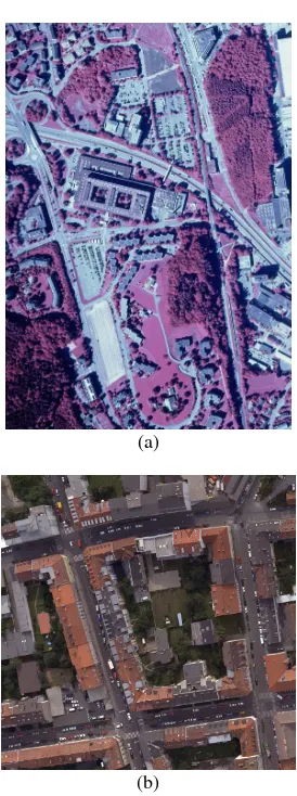
In this work two datasets have been used in the experimental evaluation (see Fig. 1). The first dataset (KLOTEN) consists of an analogue aerial image recorded with a Wild RC30 analogue
camera and shows a part of Kloten airport near Zurich, Switzerland. The image has three spectral bands in red, green and near infrared, and 15894 by 15708 pixels, which at a GSD of ~8cm correspond to the area of ~1.6 km2.
The second dataset (GRAZ) is part of a high-resolution RGB aerial image acquired with a Vexcel Ultracam D. It depicts a purely urban area of 200x200m in Graz, Austria, and has been downsampled to a GSD of ~25cm. In addition to the pixel intensities, the relative height over ground is available as a further channel. The relative height has been generated automatically by creating a DSM with dense multi-view matching, filtering it to a bare-earth DTM, and taking the difference DSM-DTM (nDSM). The height information will always be used as an additional component of the feature vector. For both datasets no pre-processing of the measured intensities was used before feature extraction.
In our evaluation we concentrate on a small number of dominant land-cover classes to ensure that a reasonable number of training and test examples are available for each class. For KLOTEN, the six classes are forest, crops, grass, buildings, roads and shadows. For GRAZ, the four classes used are buildings, roads, grass and trees. For the both datasets ground truth was annotated manually. The ground truth for the KLOTEN data consists of selected image patches for each land-cover class. For the GRAZ dataset the entire image has been annotated.
(a)
(b)
Figure 1. KLOTEN (a) and GRAZ (b) datasets.
3. METHODS 3.1 General-purpose features
Several standard feature sets were evaluated, which are widely used to classify image data, namely raw pixel intensities alone as well as augmented with NDVI and PCA channels, raw pixel patches of 9x9 pixel neighbourhoods and multi-scale texture filter responses.
Raw pixel values
The most elementary feature set is made up by the raw pixel values at each pixel, i.e. the red/green/near infrared channels for the KLOTEN dataset, respectively the red/green/blue channels for the GRAZ data. Thus the dimension of the feature vectors is three. are used to form a 7-dimensional feature vector. For the GRAZ dataset, for which no infrared channel is available, a “pseudo-NDVI” with the green and red channels was computed. Note that the projection onto the PCA-basis of the training examples is already a “data-driven method” which allows minimal adaptation to the specific data. Note however that the widely used per-pixel PCA projection is different from the PCA-features listed below.
Texture filters
As a typical “educated guess” from computer vision, which also includes neighbourhood information, we use the responses to a set of filters adopted from (Winn et al., 2005). The filter-bank consists of Gaussian filters, x- and y-scaled Gaussian derivatives, and Laplacian of Gaussians, all at multiple scales. The filters are applied separately in each spectral band to yield a 17/33 (KLOTEN) or 18/34 (GRAZ) -dimensional feature vector.
3.2 Data-driven feature extraction methods Principal Component Analysis
Feature learning aims to find a mapping, which optimally represents the data while suppressing noise. A standard method for that purpose is a linear projection onto an orthogonal basis found with Principal Component Analysis (PCA) basis. Under the assumption of i.i.d. Gaussian noise PCA finds the linear basis that is optimal in the sense that for a given number of basis vectors it preserves the largest amount of the variance in the data. The PCA approach for extracting image features is long-standing and widely used (e.g. “eigenfaces” in Turk and Pentland, 1991). In our study, we again start from the 9x9 pixel neighbourhood and project the 243 intensity values onto a 60-dimensional basis. Here, and in the remainder of the paper, we opt for a rather high dimensionality, since the random forest classifier inherently performs feature selection and is known to cope well with spurious dimensions. Thus we prefer to have too many dimensions rather than too few.
Deep belief networks
The main limitation of PCA is that the features are still a linear combination of the input, while non-linear combinations of the image data are potentially useful to highlight certain classes (probably the most well-known non-linear feature at the single-pixel level is the NDVI). Unfortunately, when the feature layers. The first layer takes the observation data as an input and converts them to features by applying a linear mapping (a contrastive divergence was used as an optimization method to find the parameters of linear mapping) followed by a sigmoid-like non-linear transformation. The next layer then takes the resulting features as an input and processes them in the same way, which yields higher-level features, and so on. Although the multi-layer architecture is maintained, the layers can be learned one after another, which simplifies the optimization problem. We rely on a publicly accessible prototype implementation of the DBN framework (Salakhutdinov, 2011). Layered sequential learning has been successfully employed for classifying images of handwritten digits. We are only aware of one work where deep belief networks have been applied to a remote sensing application, namely the binary classification of road vs. non-road pixels (Mnih, 2010).
In our experiments we have used the DBN consisting of three layers with 60 nodes in the first and second layer and 240 in the third one (the inventors recommend a top layer that is four times larger than lower ones). The batch size used for learning the network was set to 100 and the number of epochs to 500. This choice has been proved by performing a detailed evaluation of DBN parameters (number of nodes in each layer, batch size, number of epochs). For the unsupervised training of the network we have used the 9x9 pixel neighbourhood training patches. We have tested each intermediate representation, regarding it as a separate feature set: the (linear) filters of the first layer (L1), the output of mapping them with the sigmoid (L1n), and similar for the second (L2, L2n) and third levels (L3, L3n). All together we thus evaluate 6 different sets of DBN features with 60 dimensions (levels 1 and 2), respectively 240 levels.
Figure 2. Examples of the L1 filter responses
Figure 3. Feature vectors for each of the methods. The height information is used as an additional feature in the GRAZ
dataset.
3.3 Random Forest classifier
Random Forests (Breimann, 2001) are a state-of-the-art discriminative statistical classification method. They have been successfully applied to image classification tasks in remote sensing as well as other image classification tasks, e.g. (Gislason et al., 2006; Marée et al., 2005; Lepetit et al. 2006). Their popularity is based mainly on the fact that they are inherently suitable for multi-class problems, as well as on their computational efficiency during both training and testing.
A random forest is simply an ensemble of randomized decision trees. During training, the individual trees are grown independently in a top-down manner, using a subset of training examples randomly sampled from the overall training set. The internal decision nodes of the trees are learned such that they best separate the training samples according to some quality measurement (e.g. the Gini index or the information gain, typically also maximized with random sampling). Consequently, each leaf node of a tree corresponds to an estimate of the probability distribution P(k|x) over the available classes 1…k, for those samples x which reach that leaf node.
The final class probability P(k|x) is then obtained by averaging (weighted voting) over all T trees of the forest,
(1)
At test time, the test sample (represented by its feature vector) is propagated through each tree until a leaf is reached, the class probability P(k|x) is computed, and the sample is assigned to the class with the highest probability.
A random forest has only two parameters, both of which are relatively easy to set: the number of trees T, and the depth of the trees D. Both can be set conservatively: a too high T will increase computation times (unless the trees are evaluated in parallel, which is easy to implement), but not impair the results; a too high D could cause overfitting, which can however to a large extent be prevented by appropriate stopping criteria for the growing process. Empirically, the performance of random
forests is on par with other modern discriminative techniques like support vector machines or boosting of shallow trees, and significantly better than that of individual decision trees.
4. RESULTS 4.1 Comparison of different image features
For the KLOTEN dataset 64 polygons containing 1.1 Mega-pixels were used to train the classifier, and an independent sample of 103 polygons containing 9.7 Mega-pixels was used to assess the mapping accuracy.
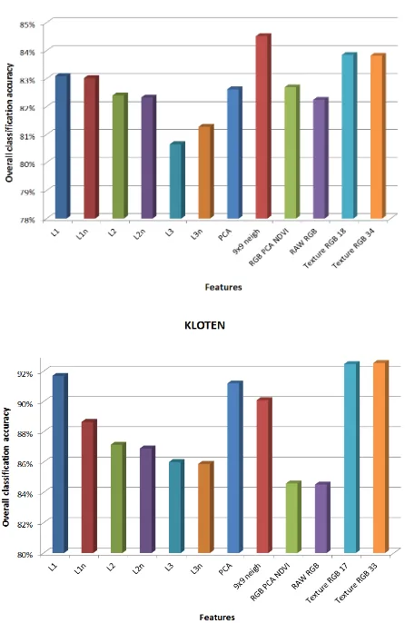
For the Graz dataset, which is fully labelled, the image was split into subsets: a training dataset consisting of 0.15 Mega-pixels and a test dataset consisting of 0.47 Mega-pixels. In order to assess the classification accuracy, confusion matrices were used. Overall classification accuracy, mapping accuracies per class and the percentage of omission and commission errors per class were then extracted from the confusion matrices (Tab. 1). The graph (Fig. 4) shows the comparison of the overall classification accuracy for all feature sets and both datasets.
In all experiments the raw classification was assessed without post-processing such as majority filtering, morphological cleaning etc. In this way biases due to the post-processing are avoided.
Figure 4. Overall classification accuracies. T = 50, D = 15. Please note the different scales on the y-axis.
Table 1. Example of the confusion matrix for 9x9 pixel neighborhood, T = 50, D = 15, GRAZ dataset
Several conclusions can be drawn from the experiments: first of all, methods based on patches dominate those based on individual pixels, which confirms the expectation that the grey-value distribution in the local neighbourhood (the “texture”) holds important information in high-resolution images and should be accounted for.
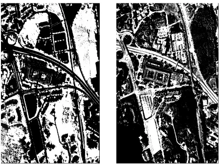
(a) (b)
Figure 5. GRAZ dataset: Ground truth (a) and classified data using 9x9 neighborhood features (T = 50, D = 15). Please note
that this depicted result is “biased” - in order to produce the classified image, the classifier has been tested on the whole
dataset (including subset for training) (b)
Regarding statistical feature learning, the conclusions are less clear. In general, complex non-linear learning does not seem to help – the best DBN features are L1 (level 1 before the non-linearity), i.e. simple linear filters. Still they slightly outperform PCA on both datasets, which hints at non-Gaussian noise. We did not manage to get the higher levels of DBN features to match the performance of linear methods. The overall lower performance on the Graz dataset may be due to the much smaller amount of training data, although further research is required to confirm this.
In terms of both the pixel-based and the patch-based features, the differences between raw intensity values and derived features are relatively small. This provides evidence that the random forest classifier is in fact able to extract the information from the raw data and feature extraction as a pre-processing step may not be required at all. E.g. the “augmented” features including the NDVI bring no improvement in the KLOTEN example although a qualitative visual check confirms that as expected it discriminates vegetation very well, and better than the raw channels. Apparently the classifier successfully recovers the information from the raw intensities.
4.2 Influence of classifier
The evaluation has shown that by and large, the random forest classifier is able to deal with raw observation data and extract
almost as much information from them as from other less basic features. This raises the question how the classifier itself should be tuned. A random forest has two main parameters, the number of trees T and the depth of the trees D (see section 3.3). In the following we test their influence on the classification result. As already mentioned, the more important thing is not to set them too low, whereas too many trees, and to a large degree also too high maximum depth, should be less critical in terms of performance. Still, overly high values naturally increase the computation time during for both training and testing,
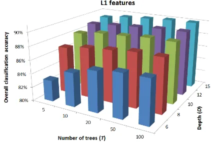
The literature suggests that using less than 5 trees is not appropriate – the averaging over very few trees will no longer have the desired regularization effect. On the other hand, rather deep trees can be trained if a lot of training data is available, which is the case in our study (>150’000 samples for GRAZ and even >1’090’000 samples for KLOTEN). We have evaluated the classifier for maximum depths of 6, 8, 10, 12, 15. Note, that depth 15 already corresponds to up to 215=32’768 possible estimates per decision tree. Tree growing stops if too few samples reach a node or if no improvement is possible at a node. We have also varied the number of trees over the range 5, 10, 20, 50, 100. The evaluation has been carried out on the KLOTEN dataset with the DBN L1 features, which are among the top performers on that dataset.
Figure 6 shows the results of the experiment. As predicted by the theory, increasing both D and T continuously improves the classification result, and both parameters eventually saturate. Increasing the number of trees does not yield further gains. Increasing the depth of a naïve implementation much further eventually leads to a performance loss, since not enough data is available to train trees of depth, say, 25 (corresponding to >33.5 million possible outcomes). In practice the performance also saturates, since splits which do not decrease the entropy of the posterior distribution are rejected, and the trees do not actually reach the maximum depth. From the evaluation we conclude that setting T = 50, D = 15 is appropriate, and all experiments described above have used these setting.
Figure 6. Overall classification accuracy in regard to random forest classifier parameters (T and D)
5. CONCLUSIONS
The aim of the present study has been to evaluate the influence of different image features on land-cover classification in images of high spatial resolution (and consequently low spectral resolution). The focus has been on urban scenes, where the high resolution is required, and also more readily available. The
evaluation was performed using two different datasets, one recorded in the R/G/NIR channels at 8 cm GSD, and one with the visible R/G/B channels plus the relative height over ground, at 25 cm GSD.
Eleven different feature sets have been tested in conjunction with the same standardized random forest classifier. Some were popular all-purpose feature sets, whereas other were learned from the images in an unsupervised, data-driven manner, to allow for adaptations to the specific data characteristics.
The main result at this stage is that features describing a larger neighbourhood around a pixel outperform those which only use the local information at the pixel itself. Furthermore, the random forest classifier is exceptionally good at extracting the necessary information even from raw intensities, such that more involved feature extractors only lead to small improvements. Finally, complex non-linear feature learning did not help. At least in our experiments we did not manage to beat simple linear feature extraction by adding non-linear processing layers. Further research is needed to reach firm conclusions and eventually give clear guidelines for feature design.
Many further tests are possible. One interesting question is whether with a simpler standard classifier raw intensities would still work as well, or whether advanced feature extraction then becomes more important. Another open question is how suitable the class probabilities estimated from different features are for further processing, e.g. smooth labelling with conditional random fields, which is known to significantly improve classification of high-resolution images.
6. REFERENCES
Bishop, C. M., 2006. Pattern Recognition and Machine Learning. Springer Verlag.
Bradley, P. S., Mangasarian, O. L., 1998. Feature selection via concave minimization and support vector machines. International Conference on Machine Learning.
Breimann, L., 2001. Random Forests. Machine Learning 45(1).
Cortes, C., Vapnik, V., 1995. Support vector networks. Machine Learning 20(3).
Dalal, N., Triggs, W., 2005. Histograms of oriented gradients for human detection. IEEE Conference on Computer Vision and Pattern Recognition.
Dalla Mura, M., Benediktsson, J. A., Waske, B., Bruzzone, L., 2010. Extended profiles with morphological attribute filters for the analysis of hyperspectral data. International Journal of Remote Sensing 31(22).
Dauchbechies, I., 1992. Ten lectures on wavelets. Society for Industrial and Applied Mathematics.
Fogel, I., Sagi, S., 1989. Gabor filters as texture discriminator. Biological Cybernetics 61(2).
Freund, Y., Shapire, R. E., 1995. A decision-theoretic generalization of the on-line learning and an application to boosting. European Conference on Computational Learning Theory.
Gehler, P. V., Nowozin, S., 2009. On Feature Combination for Multiclass Object Classification. IEEE International Conference on Computer Vision.
Gislason, P. O., Benediktsson, J. A., Sveinsson, J. R., 2006. Random forests for land cover classification. Pattern Recognition Letters 27.
Hastie, T., Tibshirani R., Friedman, J., 2009. The Elements of Statistical Learning: Data Mining, Inference and Prediction. Springer Verlag
Heikkilae, M., Pietikainen, M., Schmid, C., 2009. Desctiption of interest regions with local binary patterns. Pattern Recognition 42(3).
Hinton, G. E., Salakhutdinov, R. R., 2006a. Reducing the dimensionality of data with neural networks. Science 313(5786).
Hinton, G. E., Osindero, S., Teh, Y., 2006b. A fast learning algorithm for deep belief nets. Neural Computation 18
Kluckner, S., Mauthner, T., Roth, P. M., Bischof, H., 2009. Semantic classification in aerial imagery by integrating appearance and height information. Asian Conference on Computer Vision.
Lepetit, V., Fua, P., 2006. Keypoint recognition using randomized trees. IEEE PAMI 28(9).
Marée, R., Geurts, P., Piater, J., Wehnkel, L., 2005. Random Subwindows for Robust Image Classification. International Conference on Computer Vision and Pattern Recognition.
Mnih, V., Hinton, G. E., 2010. Learning to detect roads in high-resolution aerial images. European Conference on Computer Vision.
Salakhutdinov, R. R., 2011: Matlab Code for learning Deep Belief Networks. http://www.mit.edu/~rsalakhu/software.html
Shotton, J., Winn, J., Rother, C., Criminisi, A., 2006. TextonBoost: Joint Appearance, Shape and Context Modeling for Multi-Class Object Recognition and Segmentation. European Conference on Computer Vision.
Turk, M., Pentland, A., 1991. Eigenfaces for recognition. Journal of Cognitive Neuroscience.
Walk, S., Majer, N., Schindler K., Schiele, B., 2010. New featires and insights for pedestrian detection. IEEE Conference on Computer Vision and Pattern Recognition.
Waske, B., Benediktsson, J. A., Arnason, K., Sveinsson, J. R., 2009. Mapping of hyperspectral AVIRIS data using machine learning algorithms. Canadian Journal of Remote Sensing 35(1).
Winn, A., Crimisi, A., Minka, T., 2005. Object Categorization by learned universal visual dictionary, IEEE International Conference on Computer Vision.
Viola, P. A., Jones, M. J., 2001. Robust real-time face detection. International Conference on Computer Vision.
Yang, X., 2011. Urban Remote Sensing: Monitoring, Synthesis and Modeling in the Urban Environment. Wiley-Blackwell.