ACCURACY ANALYSIS OF A LOW-COST PLATFORM FOR POSITIONING AND
NAVIGATION
S. Hofmann, C. Kuntzsch, M. J. Schulze, D. Eggert, M. Sester
Institut f¨ur Kartographie und Geoinformatik Leibniz Universit¨at Hannover Appelstr. 9A, 30167 Hannover, Germany
{hofmann, kuntzsch, schulze, eggert, sester}@ikg.uni-hannover.de http://www.ikg.uni-hannover.de
KEY WORDS:LIDAR, robotics, accuracy analysis, close range, mapping, feature
ABSTRACT:
This paper presents an accuracy analysis of a platform based on low-cost components for landmark-based navigation intended for research and teaching purposes. The proposed platform includes a LEGO MINDSTORMS NXT 2.0 kit, an Android-based Smartphone as well as a compact laser scanner Hokuyo URG-04LX. The robot is used in a small indoor environment, where GNSS is not available. Therefore, a landmark map was produced in advance, with the landmark positions provided to the robot. All steps of procedure to set up the platform are shown. The main focus of this paper is the reachable positioning accuracy, which was analyzed in this type of scenario depending on the accuracy of the reference landmarks and the directional and distance measuring accuracy of the laser scanner. Several experiments were carried out, demonstrating the practically achievable positioning accuracy. To evaluate the accuracy, ground truth was acquired using a total station. These results are compared to the theoretically achievable accuracies and the laser scanner’s characteristics.
1 INTRODUCTION
Driving autonomously requires highly accurate and reliable po-sitioning methods. In most outdoor applications, GNSS-based systems are used. For small robots, working mainly in indoor areas, GNSS is not available. Furthermore, where high position-ing accuracies are needed its accuracy would be insufficient. A possible alternative is the use of landmarks (artificial or natural). Their precise positions need to be initially known. For indoor scenes the use of planes (walls), lines (intersection of two planes, such as floor and wall) or pole-like objects, such as pillars might be suitable. Our test setup, which is used for research and teach-ing purposes, was designed to simulate a real-world scenario on an easy-to-manage scale. Such a scenario could be autonomous driving in an urban scene using available poles along the route, such as street lights, sign posts or tree trunks. Therefore, the spatial extent and the number of landmarks are limited. As a test platform, we use a robot based on a LEGO MINDSTORMS NXT 2.0 kit, which acts as a chassis and provides the interface to the servo motors. To detect the environment, a compact laser scan-ner is used as a range sensor. The robot acts in a defined area, where pole-like objects are used as landmarks. Its task is to au-tonomously calculate its position, plan its route to a target and navigate to this target. As the robot does not use an obstacle de-tection system, all obstacles need to be mapped and localization has to be very precise, in order to avoid collisions. Two major processes have to be taken into account when analyzing the po-sitioning accuracy of the robot. First of all, the accuracy of the used map has to be analyzed. Secondly, the process of feature de-tection and extraction, which finally leads to the robot’s position, has to be examined.
This paper is structured as follows: After a short overview on literature in Chapter 2, Chapter 3 describes relevant parts of the used platform, such as sensors, the landmark map and the posi-tioning algorithm. This is followed by the experimental setup in Chapter 4 and in Chapter 5 the obtained results.
2 RELATED WORK
As discussed in Chapter 1, alternatives to GNSS-based position-ing systems have to be invented, in order to reach better posi-tioning accuracies and higher reliability. Therefore, complemen-tary positioning systems, which show a good performance where GNSS fails, especially indoors, are needed. Possible solutions are map based approaches.
environments. Therefore, we submit an easy-to-handle area and low-cost sensors for testing new algorithms in our approach.
3 MOBILE PLATFORM
In the following section we give details on our self-localization approach, which allows accurate pose estimation from a single 2D laser scan profile, assuming prior knowledge about pole-shaped landmarks in the environment (provided as a landmark map). We give details on the required map properties and describe the trans-formation of the scan profile into single landmark detections, ex-traction of unique geometric patterns and map matching. This is followed by an introduction of a self-localization robot prototype built for research and teaching purposes, which is able to use the self-localization results for e.g. routing and navigation. Finally, hardware properties with relevance to the experiments are dis-cussed.
3.1 Landmark Map Generation
When designing a map for autonomous navigation different re-quirements must be considered. If the map is designed only for one specific purpose, e.g. robot indoor navigation, such condi-tions would be the choice of objects depending on the used sen-sor or the uniqueness of feature patterns (e.g. triangles). In our test scenario, we used pole-like objects as landmarks, comparable with e.g. sign posts, lamp posts or tree trunks in an outdoor sce-nario. Poles can characterized as upright structures with homo-geneous shape, diameter and position at all heights. Therefore, they can be described with simple geometric models detectable by many different types of sensors, especially laser scanners. At high resolutions the curvature of the pole’s surface can be used for detection. At lower resolutions the linear upright structure can be found by using depth-jumps. These depth-jumps can be found at all heights of the pole, independent from the scanner’s level. It has to be considered, that using only 2D scanners with a single scan plane, the plane has to be horizontally oriented (Figure 1).
Figure 1: Laser scanner scanning in one horizontal plane.
Furthermore, the 3D structure of poles can be easily encoded into a 2D map slicing the scene horizontally. Therefore, we represent the landmarks in a 2D map using only the center coordinates and the pole’s radius. In order to support the map-matching process which is needed to find the current position, groups of landmarks are used instead of single landmarks. Grouping center points forms simple patterns, e.g. triangles. These triangles are im-plicitly stored within the landmark database. As similar-shaped triangles may occur, even more in natural environments, which may lead to ambiguities during map-matching, we consider all visible triangles in order to find unique landmark constellations.
3.2 Positioning
In the following sections, the landmark detection algorithm, which has to be adapted to the used sensor and the two-stage positioning algorithm are described.
3.2.1 Landmark Detection In order to meet the requirements of a low-cost system, we used a compact 2D laser scanner, scan-ning in one horizontal plane (Figure 1). An intuitive solution to extract poles is to search for depth-jumps within the laser scan profile. When measuring distances in a horizontal plane depth-jumps will be detected if the measured range difference at two consecutive measurements exceeds a defined threshold. If depth-jumps are found on either side of an object, it is considered a pole. The radii of pole objects, which are known from the map, is used to reduce outliers by rejecting objects which appear to be smaller or wider in radius than known landmarks. In order to calculate the pole’s center coordinates, the distance and the di-rection to the center of the detected pole has to be determined. This is done by using the pole’s diameter, which is provided by the map and the measurements on the surface of the pole. The distance to the pole’s center is computed by adding the radius of the pole to the range measurement at the mean laser beam. As mean laser beam, which is used as directional measurement, the laser beam in-between the rightmost and the leftmost laser beams of a detected pole’s surface is used.
Figure 2: Diagram of depth-jumps at a single pole object.
An alternative to this relatively simple approach using only three measurements is to estimate a best fitting circle into the scan data to calculate the center of the pole. Therefore, a least squares ad-justment is implemented using a Gauss-Helmert model. It uses the functional relationship from the measured coordinates of the circle’s edgexi, yiand the radiusrconst, which is regarded as a
constant value, to the circle’s centerxm, ym:
rconst−
q
(xi−xm)
2
+ (yi−ym)
2
= 0 (1)
from the improvement vector to the contradiction vector and a matrixAdescribing the dependency from the parameters to the contradictions. The Gauss-Helmert model demands the sum of all values to be zero. For the solution, the quadratic sum of the improvement vector is minimized with additional constraints car-rying the correlatesk:
B·v+A·xˆ+w= 0
vT·Q−1
ll ·v+ 2·k T·(
B·v+A·ˆx+w)→min (2)
As there is no stochastic information available for the measured points, the cofactor matrixQllis set as the unit matrix. The de-mands of Equation (2) lead to the following equation system:
The solution of Equation (3) leads to the unknown circle center coordinatesˆxand via variance propagation to their stochastic in-formationΣxx.
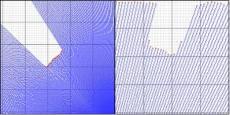
Before carrying out further experiments, the results of the circle adjustment were analyzed. However, the results obtained were not satisfying. As shown in Figure 3, scan points which belong to a landmark, do not represent the surface’s curvature due to the de-pendence of the laser scanner range measurement error on the in-cidence angle (Section 3.4), which is different for all laser beams on the (circular) pole surface. Therefore, in most cases the adjust-ment did not lead to a reliable result. This could be resolved by using the pole’s diameter known from the landmark map within the equation (instead of determining the diameter in the adjust-ment). As the circle fitting approach does not give better results, all experiments were carried out using the straight-forward pole center estimation method.
Figure 3: Scan lines plotted for a pole with 110 mm diameter at different distances to sensor (left: approx. 500mm, right: approx. 1500 mm).
3.2.2 Landmark-based Positioning Positioning in our case is a two-stage process. After finding corresponding poles among all extracted landmarks and the reference in the map (map match-ing), a least squares adjustment is used to estimate the laser scan-ner’s location. The map matching approach is based on groups of landmarks (or 2D points as their projections onto a horizon-tal plane) which form unique patterns, such as triangles. In the correlation step triangles are matched between the landmark map and the extracted pole configuration at the current position to find corresponding poles.
The reference map defines the global coordinate system and con-tains all reference poles and thus implicitly the reference trian-gles. Coordinates of all extracted poles are computed in a local robot coordinate system. The side lengths of the triangles, formed by the extracted poles are then computed using the coordinates of
all detected poles. In the following, the side lengths of local and reference triangles are compared pair-wise. All triangle pairs are rated based on a similarity score, which is defined as:
score(tmap, tscan) = (¯a(tmap)−a(t¯ scan))
starting at the shortest edge denoted with¯a, naming the remaining edges clockwise with¯bandc¯respectively.
Depending on the number of detected poles, three cases have to be considered. Firstly, the standard case, where exactly three poles are detected. Similarity scores between all reference tri-angles and the single local triangle are computed. The reference poles with the lowest squared position deviation are used as cor-responding poles. Secondly, when more than three poles are vis-ible, the algorithm starts with a single local triangle. The simi-larity score for all reference triangles is computed and as in the standard case, the best matching reference triangles is chosen to estimate the scanner’s position. Based on this result, all addi-tional detected poles are matched to the reference map and the residuals are computed. These steps are repeated for all possible triangles using all combinations of the detected poles. Finally, the solution with the maximum number of successfully matched poles is accepted. Thirdly, when less than three poles are de-tected, no map-matching is possible. Therefore, no position can be estimated at this stage. There are several conceivable solutions to this problem. In our test case, more pole landmarks could be used or other landmark types, such as planes should be consid-ered. On the sensor’s side the field of view could be extended using two scanner’s facing opposite directions. Another sensor based solution is to turn the robot by 180◦to face the opposite di-rection into the reverse navigation mode, driving backwards. The map-matching is followed by the position estimation of the scan-ner. For the position estimation the measurements of the scanner (distance and direction) and the reference features from the map are used. The results of the free stationing are the scanner’s posi-tion and orientaposi-tion as well as associated accuracies.
The following error equations are used to describe the functional correlation for the least squares adjustment:
di+vdi=
wheredi andϕi are the distance and directional measurement
to pole iwith coordinates Xi, Yi and the required properties
XR, YR, γ0, which are the scanner’s position and orientation.
Additional equations are added to consider the positional error of the reference map features:
Xi+vXi=Xi
Yi+vY i=Yi
(6)
All measurements are assumed to be uncorrelated.
3.3 Used Hardware Setup
laser scanner is attached on top of the robot, scans in a horizon-tal plane (parallel to the floor) and provides range information which is transmitted to the processing unit. The processing unit hosts software realizing the self-localization process using both the current laser scan profile as well as the prefabricated land-mark map. The software also acts as interface to the robot actu-ators via NXT Brick, allowing autonomous navigation through a familiar environment based on high-frequent self-localization re-sults. The landmark map is complete with regards to the objects within the environment in order to remove the requirement for an active collision detection. In order to avoid disturbing detections outside our experimental setup, we constructed a physical bound-ary of 2m by 2m. Cardboard tubes used as pole objects are placed within this box. An experiment setup requires to accurately mea-sure ground truth positions of all objects within the environment (e.g. by total station measurement), creating a landmark map and providing it to the self-localization software.
Naturally, the application of the position estimation on route plan-ning and navigation leads to further sources for error. As the fo-cus of this paper is the theoretical investigation and experimental validation of the self-positioning approach, we decided to remove as many external effects on the positioning accuracy as possible from the experiments, i.e. we performed all measurements only using the laser scanner and the self-positioning software. Move-ment of the laser scanner has been performed manually by sim-ulating a supposed trajectory and performing measurements at discrete waypoints along the route. Further details on the im-plementation of the system, routing and navigation specifics are discussed in a previous work of the authors.
3.4 Laser Scanner Characterization
For range measurements we use the Hokuyo URG-04LX laser scanner, which has been characterized regarding distance mea-surement errors under varying external preconditions (incidence angle, surface properties) by e.g. (Kneip et al., 2009, Okubo et al., 2009). For the interpretation of our experimental results, we rely on the following device characteristics described in the aforementioned literature. The device specification mentions a distance measurement error of±10mm within a measurement range between 20 mm and 1 m and±1% of the true distance for measurement distances above 1 m, though aforementioned char-acterization experiments have found the expectable error to be about±2% for distances above 1 m. The maximum distance measurable with the scanner is 4 m, which is considered within the experiments by only measuring within the physical bound-aries (dimensions 2 m by 2 m). The scanner’s field of view has an opening angle of 240◦. Regarding the angular accuracy of the measurement, (Kneip et al., 2009, Okubo et al., 2009) have found a discrepancy of about 1% between the true center of mea-surement and the center mentioned within the device specifica-tion. This error could be reduced by calibration prior to measure-ments. As this error only influences the heading component of the pose estimation and not the position and because the order of magnitude of this error is rather insignificant for the navigation task (considering the stability/positional accuracy of the device installation on top of the robot and the accuracy of mechanical navigation), we chose not to perform this calibration step. This error may, however, be reflected within the pose estimation re-sults.
For one, both characterization papers describe a significant drop in range measurement in the first 30 minutes after scanner startup (a drift effect, stabilizing afterwards). We considered this prop-erty by having a long enough scanner startup phase before all measurements. Furthermore, the relation between surface prop-erties and measurement errors have been studied in (Okubo et
al., 2009). They conclude, that sensor specifications are valid for white paper tests with higher errors for different color, light-ness and reflectivity properties. The pole objects used within our experiments are made of cardboard, falling into the matted col-ors/gray level category (average distance measurement error of about 30 mm). Another property of the scanner is a relation be-tween distance measurement error and laser incidence angle on the object surface. As the used pole objects have circular foot-prints, its laser-scan profile consists of (near) orthogonal mea-surement an several, increasing incidence angles towards both sides of the pole. This leads to increasing measurement errors for surface range measurements which in turn leads to an erro-neous measurement of the 2D shape of the pole surface, which significant decreases the quality of curve fitting approaches for pole center estimation (discussed in detail in section 3.2.1). Ad-ditionally, we have to deal with the unknown optic center of the device which is not specified by the manufacturer. Similar to the approach taken by other authors, we assume the optic center to coincide with the geometric center of the device case.
Although (Kneip et al., 2009, Okubo et al., 2009) developed first coarse calibration models for distance measurement correction (under several assumptions regarding external preconditions), we chose not to reprocess measured distances. All measurements will directly reflect measured distances including systematic de-vice specific errors. However, we would expect the achievable accuracy of the self-positioning approach to increase in perfor-mance when coupled with a proper calibration for specific ex-ternal preconditions, as it is closely dependent on the distance measurement accuracy.
4 EXPERIMENTS
Our experiments are divided into two main parts. Firstly, mea-surements to determine the accuracy of single landmarks have to be carried out. Secondly, the subsequent positioning accuracy, which mainly depends on the extracted landmarks, can be ana-lyzed.
4.1 Landmarks
The positioning accuracy of our used platform is to a large extend depending on highly accurate landmark positions, which are, in our case, the center points of the used poles. Several tests were carried out to evaluate the accuracy of the distance to the pole’s center based on the two variable object parameters - pole diam-eter and distance to the sensor. Therefore, measurements with different pole diameters at different distances were carried out. Based on this measurements, the poles center was calculated us-ing the mean laser beam based on the used depth-jump algorithm in comparison to the results of a best fitting circle. We expect the latter to give better results, as the adjustment calculation takes more measurements on the pole’s surface into consideration com-pared to the calculation using only the two outmost laser beams of the pole (Figure 2). In order to analyze the dependency on the distance from sensor to object, two sample distances were chosen with respect to the limited test area. In the experiments, we evaluated two different pole diameters of 45 mm and 110 mm. As reference, the scanner’s position and the pole’s center coor-dinates and thus implicitly the distance to the pole’s center were surveyed using a total station. The resulting positional accuracies of the reference landmarks, with a standard deviation of 1.3 mm.
4.2 Position
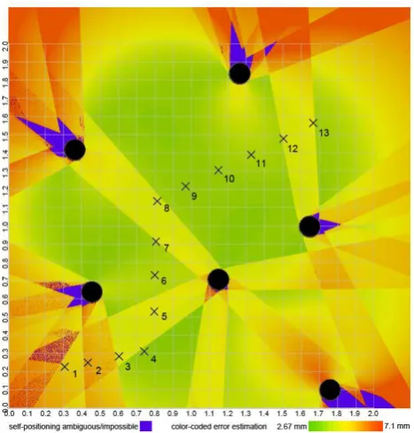
Therefore, a scanner with a 360◦angle of view was simulated in order to eliminate directional dependencies. The map area was decomposed in a discrete raster and subsequently, the possible positioning accuracy was calculated for every cell based on the landmark geometry, visibility conditions and the a priori racies (Figure 4). The theoretically achievable positioning accu-racy indicated by colors from red (7.1 mm) to green (2.67 mm). Blue indicates regions where no positioning is possible, because less than the necessary three landmarks are visible. Doted blue regions indicate areas where ambiguities exist, which means no unique landmark constellation was detected. This can be solved by introducing a filter algorithm such as Kalman Filter to take prior positions into account. In comparison with the simulated accuracy color map, the positioning accuracies are expected to be lower in some areas due to occluded poles caused by the limited angle of view of240◦. The theoretically achievable positioning accuracy is determined in the least squares adjustment for all po-sitions with more than three poles visible.
Figure 4: Accuracy color map for one landmark constellation (gray circles) and example trajectory.
For our experiments a route was chosen exemplarily and decom-posed into discrete points, which are assumed to be drivable in both directions. At these discrete points all following measure-ments were carried out, in order to determine the positioning ac-curacy. In the following, the positioning accuracy is split into two parts. First of all, the repeatability of the localization at a certain position was evaluated. Therefore, the position was cal-culated several times based on the respective scan profiles as each scan profile leads to a single position. The resulting point distri-bution could then be analyzed. Secondly, for localization and the navigation based on it, the absolute positioning accuracy is even more important. In our test set up, we placed the scanner on 13 positions at roughly equal distance along the test route. For every point, the position was calculated in two directions, the scanner facing forward and backwards. Additionally, at the turn-ing points, where the platform would have to change its drivturn-ing direction to follow the route, four poses were determined, using all four possible orientations. Reference positions for the scanner were surveyed as ground truth for every scanner’s position along the trajectory using a total station. Therefore, the center point of
the scanner’s casing was used as reference point.
5 RESULTS AND DISCUSSION
In this chapter the determined accuracy of a single detected land-mark as well as the positioning accuracy of the scanner is dis-cussed.
5.1 Landmark Measurement Accuracy
The parameters describing a landmark from the scanner’s point of view are distance and direction to the pole’s center. In our ex-periments we analyzed the distance measurements to the pole and subsequently to the pole’s center and the resulting center coordi-nates. The resulting distances to the pole’s center are exemplarily evaluated for two types of poles (diameter 45 mm and 110 mm) at two different distances. The reached accuracy of determining the distance to the pole’s center using the in section 3.2.1 described depth-jump algorithm is in the range of 3-20 mm depending on the measuring distance. This results agree well with the theoreti-cal expectations, due to the absence of theoreti-calibration.
5.2 Positioning Accuracy
The positioning accuracy was determined at discrete positions along a defined route. It includes parts were positioning is only possible in one driving direction and other parts were position-ing is possible in both directions. At two points, the position is determined based on four different orientations, when the driving direction changes.
Figure 5: Example trajectory with landmarks. Reference po-sitions are marked as black cross, starting at position 1, green marks forward positions and red backwards positions. Blue and magenta indicate additional directions at turning points.
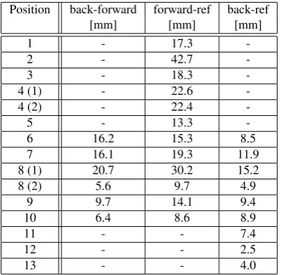
For positioning in a real world scene and autonomous navigation the absolute position might be more important. Therefore, we compared the calculated positions from the laser scanner’s mea-surements with ground truth for all scanner’s positions. The re-sults are in the range of 2.5 mm to 30 mm at positions, where only three poles are visible. Table 1 presents the experimental results at five chosen positions, where at least two scanning orientations were used to determine its position. At all other positions only one orientations led to a localization result due to too many oc-cluded poles. At point 8 four scanning directions were used. The number of visible poles was three or more, exactly three poles could be detected at position 7 (forward) and 8 (all). In compari-son, the theoretically achievable accuracy for the evaluated posi-tions given by the adjustment, with more than three poles visible, is between 2.9 mm and 5.1 mm.
Figure 6: Deviation of calculated positions based on different scans. Different colors show different scanner orientations (black cross: reference position).
Position back-forward forward-ref back-ref
[mm] [mm] [mm]
1 - 17.3
-2 - 42.7
-3 - 18.3
-4 (1) - 22.6
-4 (2) - 22.4
-5 - 13.3
-6 16.2 15.3 8.5
7 16.1 19.3 11.9
8 (1) 20.7 30.2 15.2
8 (2) 5.6 9.7 4.9
9 9.7 14.1 9.4
10 6.4 8.6 8.9
11 - - 7.4
12 - - 2.5
13 - - 4.0
Table 1: Differences at pole centers. (back-forward): between the opposite scanner directions at same position. (forward-ref) and (backward-ref): between reference and estimated scanner posi-tion. (1) and (2) indicate positions 4 and 8 as turning points with four possible orientations.
Compared to the low distance measurement accuracy of the used scanner (section 3.4) our experiments lead to a positioning accu-racy within 1 cm to 3 cm, which means 2% error with regard to the maximum measuring distance at our test area. A calibration
of the scanner with respect to the given setup could reduce the scanner’s systematic errors, such as the dependence on surface properties or incidence angles at detected poles.
6 CONCLUSIONS AND FUTURE WORK
In this paper, we introduced a self-localization approach based on landmark-maps. After giving insight on the theoretical accuracy of the approach for an exemplary landmark setup, we conducted a series of experiments demonstrating the practically achievable accuracy using a robot prototype based on a Hokuyo URG-04LX laser scanner. This includes a detailed discussion of possible error resulting from the chosen hardware and experimental setup.
Our experiment results (maximum errors of about±2% of the greatest measured distance within the experimental setup) verify that the self-localization accuracy is well within the order of mag-nitude of the various input errors (mainly distance measurement error of the laser scanner). We consider the obtained accuracy sufficient for more complex tasks relying on an accurate position estimation (e.g. autonomous navigation within a well-known en-vironment).
Finally we made several propositions for possible improvement of the self-localization result by applying a calibration model on the range measurements of the laser scanner (reducing effects of object surface properties, incident angles and device heading).
REFERENCES
Blervaque, V., 2008. Prevent maps and adas d12.1 final report. Technical report, ERTICO ITS Europe, http://www.prevent- ip.org/download/deliverables/MAPS&ADAS/PR-12100-DEL-080127-v10-ERT-D12.1%20MAPS&ADAS%20Final%20Report.pdf (last accessed on January 3, 2012).
Brenner, C., 2009a. Extraction of features from mobile laser scanning data for future driver assistance systems. In: Ad-vances in GIScience: Proceedings of 12th AGILE Conference on GIScience, Lecture Notes in Geoinformation and Cartography, Springer, pp. 25–42.
Brenner, C., 2009b. Global localization of vehicles using local pole patterns. In: DAGM 2009, 31st Annual Symposium of the German Association for Pattern Recognition, LNCS 5748, pp. 61–70.
Burgard, W. and Hebert, M., 2008. Springer Handbook of Robotics. Springer, chapter World Modeling, pp. 853–869.
Hu, H. and Gu, D., 2000. Landmark-based navigation of indus-trial mobile robots. International Journal of Industry Robot Vol. 27, pp. 458 – 467.
Kneip, L., Tache, F., Caprari, G. and Siegwart, R., 2009. Char-acterization of the compact hokuyo URG-04LX 2d laser range scanner. In: Robotics and Automation, 2009. ICRA ’09. IEEE International Conference on, pp. 1447–1454.
Okubo, Y., Ye, C. and Borenstein, J., 2009. Characterization of the hokuyo urg-04lx laser rangefinder for mobile robot obstacle negotiation. In: Proc. SPIE 7332.
Thrun, S., Burgard, W. and Fox, D., 2005. Probabilistic Robotics. The MIT Press, Cambridge, Mass.