john strauss et al indonesian living standards before and after the financial crisis evidence from the indonesia family life survey

(1)

from฀

www.rand.org

฀as฀a฀public฀service฀of฀

the฀RAND฀Corporation.

6 Jump฀down฀to฀document

Purchase฀this฀document

Browse฀Books฀&฀Publications

Make฀a฀charitable฀contribution

Visit฀RAND฀at฀

www.rand.org

Explore฀

RAND฀Labor฀and฀Population

฀

View฀

document฀details

This฀ document฀ and฀ trademark(s)฀ contained฀ herein฀ are฀ protected฀ by฀ law฀ as฀ indicated฀ in฀ a฀ notice฀ appearing฀ later฀ in฀ this฀ work.฀ ฀ This฀ electronic฀ representation฀ of฀ RAND฀ intellectual฀ property฀ is฀ provided฀ for฀ non-commercial฀use฀only.฀฀Permission฀is฀required฀from฀RAND฀to฀reproduce,฀or฀ reuse฀in฀another฀form,฀any฀of฀our฀research฀documents.

Limited฀Electronic฀Distribution฀Rights

For฀More฀Information

Support฀RAND

CHILDREN฀AND฀ADOLESCENTS

CIVIL฀JUSTICE

EDUCATION

ENERGY฀AND฀ENVIRONMENT

HEALTH฀AND฀HEALTH฀CARE

INTERNATIONAL฀AFFAIRS

POPULATION฀AND฀AGING

PUBLIC฀SAFETY

SCIENCE฀AND฀TECHNOLOGY

SUBSTANCE฀ABUSE

TERRORISM฀AND฀ HOMELAND฀SECURITY

TRANSPORTATION฀AND INFRASTRUCTURE

U.S.฀NATIONAL฀SECURITY

(2)

(3)

(4)

The RAND Corporation is a nonprofit research organization providing objective analysis and effective solutions that address the challenges facing the public and private sectors around the world.

RAND publications do not necessarily reflect the opinions of its research clients and sponsors. “RAND” is a registered trademark.

This product is part of the RAND Corporation’s monograph series. RAND monographs present major research findings. All RAND monographs undergo rigorous peer review to ensure high standards for research quality and objectivity.

The Institute of Southeast Asian Studies (ISEAS) was established as an

autonomous organization in 1968. It is a regional centre dedicated to the study of socio-political, security and economic trends and developments in Southeast Asia and its wider geostrategic and economic environment.

The Institute’s research programmes are the Regional Economic Studies (RES, including ASEAN and APEC), Regional Strategic and Political Studies (RSPS), and Regional Social and Cultural Studies (RSCS).

(5)

Indonesian

Living Standards

Before and After the Financial Crisis

John Strauss • Kathleen Beegle • Agus Dwiyanto • Yulia Herawati Daan Pattinasarany • Elan Satriawan • Bondan Sikoki Sukamdi • Firman Witoelar

UNIVERSITY OF GADJAH MADA Yogyakarta

LABOR AND POPULATION

Center for the Study of the Family in Economic Development

(6)

First published in Singapore in 2004 by Institute of Southeast Asian Studies 30 Heng Mui Keng Terrace Pasir Panjang

Singapore 119614

E-mail: publish@iseas.edu.sg

Website: http://bookshop.iseas.edu.sg

First published in the United States of America in 2004 by RAND Corporation

1700 Main Street, P.O. Box 2138 Santa Monica, CA 90407-2138 USA

To order through RAND Corporation or to obtain additional information, contact Distribution Services: Tel: 310-451-7002; Fax: 310-451-6915; E-mail: order@rand.org All rights reserved. No part of this publication may be reproduced, stored in a retrieval system, or transmitted in any form or by any means, electronic, mechanical,

photocopying, recording or otherwise, without the prior permission of the Institute of Southeast Asian Studies and RAND Corporation.

The responsibility for facts and opinions in this publication rests exclusively with the authors and their interpretations do not necessarily reflect the views or the policy of the Institute, RAND Corporation or their supporters.

ISEAS Library Cataloguing-in-Publication Data

Indonesian living standards before and after the financial crisis / John Strauss ... [et al.]. 1. Cost and standard of living—Indonesia.

2. Wages—Indonesia.

3. Poverty—Indonesia.

4. Education—Indonesia.

5. Public health—Indonesia.

6. Birth control—Indonesia.

7. Household surveys—Indonesia.

I. Strauss, John,

1951-HD7055 I412 2004

ISBN 981-230-168-2 (ISEAS, Singapore) ISBN 0-8330-3558-4 (RAND Corporation)

Cover design by Stephen Bloodsworth, RAND Corporation Typeset by Superskill Graphics Pte Ltd

(7)

v

List of Figures

Fig. 1.1 Timing of the IFLS and the Rp/USD Exchange Rate 2 Fig. 1.2 Food Price Index (January 1997=100) 3

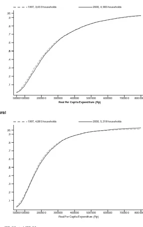
Fig. 3.1 Poverty Incidence Curves: 1997 and 2000 29 Fig. 3.2 Poverty Incidence Curves in Urban and

Rural Areas: 1997 and 2000 31

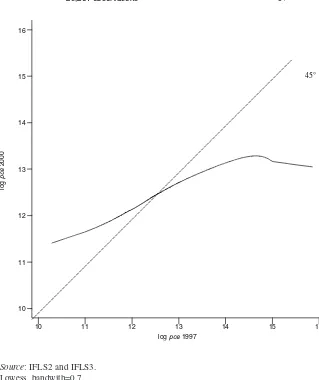
Fig. 3.3 Log Per Capita Expenditure 1997 and 2000

for Panel Individuals 43

Appendix Log Per Capita Expenditure 1997 and 2000

Fig. 3.1 for Panel Individuals in Urban and Rural Areas 54

Fig. 5.1 CDF of Market and Self-Employment Log

Wages in 1997 and 2000 for Men 87 Fig. 5.2 CDF of Market and Self-Employment Log

Wages in 1997 and 2000 for Women 88

Fig. 7.1 Adult Height by Birth Cohorts 1900–1980 136 Fig. 7.2 Child Standardized Height-for-Age, 3–108 Months 138 Fig. 7.3 CDF of Child Standardized Height-for-Age

for 3–17 Months 140

Fig. 7.4 CDF of Child Standardized Height-for-Age

Fig. 7.5 CDF of Child Standardized Height-for-Age

Fig. 7.6 Child Standardized Weight-for-Height, 3–108 Months 148 Fig. 7.7 CDF of Child Standardized Weight-for-Height

Fig. 7.8 CDF of Child Standardized Weight-for-Height

Fig. 7.9 CDF of Child Standardized Weight-for-Height

(11)

ix Fig. 7.10 CDF of Haemoglobin Level for Children

12–59 Months 157

Fig. 7.11 CDF of Haemoglobin Level for Children 5–14 Years 158 Fig. 7.12 CDF of Adult BMI for 15–19 Years 168 Fig. 7.13 CDF of Adult BMI for 20–39 Years 169 Fig. 7.14 CDF of Adult BMI for 40–59 Years 170 Fig. 7.15 CDF of Adult BMI for 60 Years and Above 171 Fig. 7.16 CDF of Blood Pressure Levels for Adult

20–39 Years 180

Fig. 7.17 CDF of Blood Pressure Levels for Adult

40–59 Years 181

Fig. 7.18 CDF of Blood Pressure Levels for Adult

60 Years and Above 182

Fig. 7.19 CDF of Haemoglobin Level for Adult 15–19 Years 197 Fig. 7.20 CDF of Haemoglobin Level for Adult 20–59 Years 198 Fig. 7.21 CDF of Haemoglobin Level for Adult 60 Years

and Above 199

Appendix CDF of Standardized Height-for-Age for Children

Fig. 7.1 Age 3–17 Months in Urban and Rural Areas 211 Appendix CDF of Standardized Height-for-Age for Children

Fig. 7.2 Age 18–35 Months in Urban and Rural Areas 212 Appendix CDF of Standardized Height-for-Age for Children

Fig. 7.3 Age 36–59 Months in Urban and Rural Areas 213 Appendix CDF of Standardized Weight-for-Height for Children Fig. 7.4 Age 3–17 Months in Urban and Rural Areas 214 Appendix CDF of Standardized Weight-for-Height for Children Fig. 7.5 Age 18–35 Months in Urban and Rural Areas 215 Appendix CDF of Standardized Weight-for-Height for Children Fig. 7.6 Age 36–59 Months in Urban and Rural Areas 216

Fig. 12.1a Probability of Receiving Aid by Per Capita

Expenditure 2000 336

Fig. 12.1b OPK Subsidy as Percent of Per Capita

Expenditure by Per Capita Expenditure 2000 336 Fig. 12.2a Government Scholarship Receipt by Log PCE

by Age of Enrolled Children 351 Fig. 12.2b Government Scholarship Receipt by Log PCE

(12)

x

Appendix Probability of Receiving Aid by Per Capita

Fig. 12.1a Expenditure 2000: Urban 364 Appendix OPK Subsidy as Percent of Per Capita Expenditure

Fig. 12.1b by Per Capita Expenditure 2000: Urban 364 Appendix Probability of Receiving Aid by Per Capita

Fig. 12.2a Expenditure 2000: Rural 365 Appendix OPK Subsidy as Percent of Per Capita Expenditure

(13)

xi

List of Tables

Appendix Number of Communities in IFLS 13 Table 2.1

Appendix Household Recontact Rates 14

Table 2.2

Appendix Type of Public and Private Facilities and Schools 15 Table 2.3

Appendix Age/Gender Characteristics of IFLS and SUSENAS:

Table 2.4 1997 and 2000 16

Appendix Location Characteristics of IFLS and SUSENAS:

Table 2.5 1997 and 2000 17

Appendix Completed Education of 20 Year Olds and Above

Table 2.6 in IFLS and SUSENAS: 1997 and 2000 18 Appendix Household Comparisons of IFLS and SUSENAS:

Table 2.7 1997 and 2000 19

Table 3.1 Percent of Individuals Living in Poverty:

IFLS, 1997 and 2000 21

Table 3.2 Rice and Food Shares 1997 and 2000 24 Table 3.3 Percent of Individuals Living in Poverty for Those

Who Live in Split-off Households in 2000:

IFLS, 1997 and 2000 26

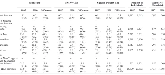
Table 3.4 Real Per Capita Expenditures: IFLS, 1997 and 2000 27 Table 3.5a Foster-Greer-Thorbecke Poverty Indices for Urban

Residence: IFLS, 1997 and 2000 32 Table 3.5b Foster-Greer-Thorbecke Poverty Indices for Rural

Residence: IFLS, 1997 and 2000 33 Table 3.6 Poverty: Linear Probability Models for 1997 and 2000 35 Table 3.7 In- and Out-of-Poverty Transition Matrix:

IFLS, 1997 and 2000 39

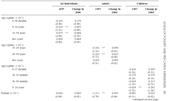
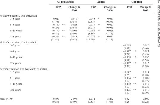
Table 3.8 Poverty Transitions for All Individuals, 1997 and 2000: Multinomial Logit Models: Risk Ratios Relative to

(14)

xii

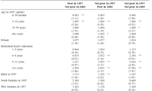
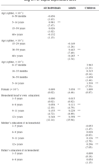
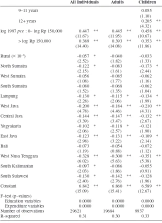
Table 3.9 Log of Per Capita Expenditure 2000 45 Appendix Poverty Lines (Monthly Rupiah Per Capita) 55 Table 3A.1

Appendix Real Per Capita Expenditure 2000 and 1997:

Table 3B.1 Test for Stochastic Dominance 58 Appendix Poverty Transitions for All Adults, 1997 and 2000:

Table 3C.1 Multinomial Logit Models: Risk Ratios Relative to

Being Poor in both 1997 and 2000 59 Appendix Poverty Transitions for All Children, 1997 and 2000: Table 3C.2 Multinomial Logit Models: Risk Ratios Relative to

being Poor in both 1997 and 2000 61

Table 4.1 Distribution of Individual’s Perception of Standard

of Living, 1997 and 2000 64

Table 4.2 Individual’s Perception on Standard of Living,

1997 and 2000 65

Table 4.3 Individual’s Perception on Quality of Life, 2000 66 Table 4.4 Linear Regression Models of Subjective Well-being 68

Table 5.1 Employment Characteristics, Adults 15–75 72 Table 5.2 Distribution of Employment by Sector, Adults 15–75 74 Table 5.3 Working for Pay (Employee or Self-employed),

Adults 15–75, Linear Probability Models 76 Table 5.4 Transitions in Work (Employee/Self-employed/

Unpaid Family Labour) by Gender and Age 77 Table 5.5 Transitions in Work by Sector and Gender,

Adults 15–75 78

Table 5.6 Transitions in Work, Men 15–75:

Multinomial Logit Models: Risk Ratios Relative

to Not Working in Either Year 79 Table 5.7 Transitions in Work, Women 15–75:

Multinomial Logit Models: Risk Ratios Relative

to Not Working in Either Year 81 Table 5.8 Median Real Hourly Wages Among Self-Employed

and Employees, Adults 15–75 84

Table 5.9 Median Real Hourly Wages by Type of Work,

Adults 15–75 84

(15)

xiii Table 5.11 Change in Log Wages (2000 wage – 1997 wage),

Adults 15–75, Linear Probability Models 89 Table 5.12 Main Activities of Children (as % of Total Number

of Children in Each Age Group) 92 Table 5.13 Children Current and Ever Work Participation

Rates by Age 93

Table 5.14 Average Hours Worked per Week for Children

Age 5–14 Who Worked 95

Table 5.15 Percentage of Children Age 10–14 Currently Working by Residence, Per Capita Expenditure,

and Type of Household 97

Table 5.16 Linear Probability Models of Current Work

Participation for Children Age 10–14 98 Appendix Transitions in Work for Pay, Men 15–75:

Table 5.1 Multinomial Logit Models: Risk Ratios Relative

to Not Working in Either Year 102 Appendix Transitions in Work for Pay, Women 15–75:

Table 5.2 Multinomial Logit Models: Risk Ratios Relative

to Not Working in Either Year 104 Appendix Log of Market and Self-Employment Wages:

Table 5.3 Test for Stochastic Dominance 106

Table 6.1 Percentage of Children Not Currently Enrolled 109 Table 6.2 School Enrolment: Linear Probability Models

Boys and Girls, 7–12 Years 111

Table 6.3 School Enrolment: Linear Probability Models

Table 6.4 School Enrolment: Linear Probability Models

Table 6.5 Hours in School Last Week, Among Those Currently

in School 115

Table 6.6 School Expenditures in Rupiah by Category,

Students 15–19 Years 116

Table 6.7 School Expenditure Models, Students 15–19 Years 117 Table 6.8 Receipt of Assistance for School Among Enrolled

Students, School Year 2000/2001 118 Table 6.9 Religious Orientation of Schools 120 Table 6.10 Enrolment Rates and Student/Teacher Ratio:

(16)

xiv

Table 6.11 Enrolment Rates and Student/Teacher Ratio:

Junior Secondary Schools 122

Table 6.12 Enrolment Rates and Student/Teacher Ratio:

Senior Secondary Schools 123

Table 6.13 Teacher Characteristics: Mathematics 125 Table 6.14 Classroom Infrastructure 126 Table 6.15 Primary School Charges 127 Table 6.16 Junior Secondary School Charges 128 Table 6.17 Senior Secondary School Charges 129 Appendix School Type Among Children

Table 6.1 Currently Enrolled 132

Table 7.1 Child Standardized Height-for-Age 139 Table 7.8 Parent- and Nurse-assessed General Health: Linear

Probability Models for Poor Health Children,

aged 0–14 years 163

Table 7.9 Adult Body Mass Index 166

Table 7.10a Adult Female Body Mass Index Regressions 174 Table 7.10b Adult Male Body Mass Index Regressions 176 Table 7.11 Adult Blood Pressure and Levels of Hypertension 178 Table 7.12a Female Blood Pressure and Levels of Hypertension

Regressions 183

Table 7.12b Male Blood Pressure and Levels of Hypertension

Regressions 185

Table 7.13 Frequency of Smoking 187

Table 7.14 Average Number of Cigarettes Smoked Per Day

(for Current Smokers) 190

(17)

xv Table 7.18 Health Conditions of Adults 203 Table 7.19 Self- and Nurse-reported General Health:

Linear Probability Models for Poor Health Adults,

Aged 15+ 204

Table 7.20 Physical Ability in Daily Activity: Linear Probability Model of Having Any Activity and OLS of Number of Activities Done Uneasily, Adults Aged 40+ 206 Appendix Child Height-for-Age:

Table 7.1 Test for Stochastic Dominance 217 Appendix Child Weight-for-Height:

Table 7.2 Test for Stochastic Dominance 219 Appendix Child Hemoglobin Level:

Table 7.3 Test for Stochastic Dominance 221 Appendix Adult Body Mass Index: Test for Stochastic

Table 7.4 Dominance for Undernourishment 223 Appendix Adult Body Mass Index: Test for Stochastic

Table 7.5 Dominance for Overweight 225 Appendix Systolic Levels: Test for Stochastic Dominance 226 Table 7.6a

Appendix Diastolic Levels: Test for Stochastic Dominance 228 Table 7.6b

Appendix Frequency of Smoking: Rural and Urban 230 Table 7.7

Appendix Average Number of Cigarettes Smoked Per Day

Table 7.8 (for Current Smokers); Rural and Urban 234 Appendix Age When Start Smoking; Rural and Urban 235 Table 7.9

Appendix Adult Haemoglobin Level:

Table 7.10 Test for Stochastic Dominance 236

Table 8.1 Use of Outpatient Healthcare Facilities by Children

in Last Four Weeks 239

Table 8.2 Use of Outpatient Healthcare Facilities by Adults

in Last Four Weeks 241

Table 8.3a Immunization Uptake for Children,

(18)

xvi

Children with Completed Immunization Uptake 256 Appendix Use of Outpatient Healthcare Facilities by Children

Table 8.1 in Last Four Weeks: Rural and Urban Areas 260 Appendix Use of Outpatient Healthcare Facilities by Adults

Table 8.2 in Last Four Weeks: Rural and Urban Areas 262 Appendix Immunization Uptake for Children,

Table 8.3 Aged 12–59 months: Rural and Urban Areas 264

Table 9.1 Provision of General Services by Type of Facilities 267 Table 9.2 Stock Outages of Vaccines During the Last Six Months

Among Those Providing, by Type of Facilities 269 Table 9.3 Provision of Drugs by Type of Facilities 271 Table 9.4a Stock Outages of Drugs at Present Among Those

(19)

xvii Table 9.7 Median Charges for the Provision of General

Services by Type of Facilities 282 Table 9.8 Median Charges for the Provision of Drugs by

Type of Facilities 284

Table 9.9 Median Charges for the Provision of Services at the Laboratory by Type of Facilities 287 Table 9.10 Provision of Services by Posyandu 288 Table 9.11 Availability of Supplies and Instruments

by Posyandu 290

Table 9.12 Median Charges for the Provision of Services

by Posyandu 291

Table 10.1 Use of Contraceptives by Currently Married Women

Aged 15–49, by Age Group 293

Table 10.2 Use of Contraceptives by Currently Married Women

Aged 15–49, by Region 296

Table 10.3 Use of Contraceptives by Currently Married Women Aged 15–49, by Years of Schooling 297 Table 10.4 Use of Contraceptives by Currently Married Women

Aged 15–49 Years: Linear Probability Models of the

Use of Contraceptives 298

Table 10.5 Source of Contraceptive Supplies Among Pill and Injection Users, Currently Married Women

Aged 15–49 301

Table 10.6 Median Charges of Contraceptive Services Among Pill and Injection Users, Currently Married Women

Aged 15–49 302

Appendix Source of Contraceptive Supplies Among Pill and Table 10.1a Injection Users Currently Married Women

Aged 15–49, by Residence 304

Appendix Source of Contraceptive Supplies Among Pill Table 10.1b and Injection Users Currently Married Women

Aged 15–49, by Regions 305

Appendix Median Charges of Contraceptive Services Among Table 10.2a Pill and Injection Users Currently Married Women

Aged 15–49, by Residence 306

Appendix Median Charges of Contraceptive Services Among Table 10.2b Pill and Injection Users Currently Married Women

(20)

xviii

Table 12.2 Prevalence of Social Safety Net Programmes in

IFLS3 Communities 323

Table 12.7 Prevalence and Value of Assistance and Subsidy

Received by Individuals 333

Table 12.8 Linear Probability Models for Receiving Assistance

and OPK Subsidy 338

Table 12.9 Linear Regressions for Value of Log Per Capita Assistance and OPK Subsidy During Last Four

Weeks, Among Those Receiving 340 Table 12.10 Prevalence of Padat Karya Programme in IFLS3

Communities 342

Table 12.11 Prevalence of PDMDKE Programme in IFLS3

Communities 344

Table 12.12 Prevalence of Scholarship Programmes

Among Schools 348

Table 12.13 Receipt of Assistance for School Among Enrolled

Students, School Year 2000/2001 349 Table 12.14 Linear Probability Models of Student Receipt of

Government Scholarship by Age Group, 2000/2001 352 Table 12.15 Prevalence of Operational Funds Assistance (DBO)

and Operational and Maintenance Funds for Schools 354 Table 12.16 Kartu Seh_at_Serv_i_{ces and Coverage by}

Type of Provider 355

(21)

xix Table 12.17 Usage of Health Card and Letter of Non-affordability

in Outpatient and Inpatient Care Visits by

Type of Provider 356

Table 12.18 Supplementary Distribution Programme (PMT) in

IFLS3 Communities 359

Table 12.19 Supplementary Food Programmes at Primary School 360

Table 13.1 Desa/Kelurah_an_Fi_nance ₃₆₉

Table 13.2 Budget and Budget Authority of Puskesmas/

Puskesmas Pembantu 371 Table 13.3 Degree of Decision-making Authority at

Puskesmas and Puskesmas Pembantu (Pustu) 374 Table 13.4 Degree of Decision-making Authority by

Institution at Puskesmas and Puskesmas Pembantu 377 Table 13.5 Schools: Decision-making Authority 381 Appendix Kelurah_an_Urban_Fi_{nance by Reg}_i_on ₃₈₄

Table 13.1a

(22)

xx

Acknowledgements

The authors would like to thank the following staff for their very important assistance in creating tables and figures: Tubagus Choesni, Endang Ediastuti, Anis Khairinnisa, Umi Listyaningsih, Wenti Marina Minza, Muhammad Nuh, Agus Joko Pitoyo, Pungpond Rukumnuaykit, Henry Sembiring and Sukamtiningsih.

The authors would also like to thank Jean-Yves Duclos, Kai Kaiser and Jack Molyneaux for very helpful discussions early in the drafting process and thanks to Tubagus Choesni, Molyneaux and the RAND Data Core for aid in obtaining the BPS data.

Thanks also to the participants of a workshop held in Yogyakarta on 2–3 July 2002, at which the first draft was extensively discussed and many suggestions made that were incorporated into the revisions. In addition to the authors, attendees included: Irwan Abdullah, I Gusti Ngurah Agung, Stuart Callison, Muhadjir Darwin, Faturochman, Johar, Kai Kaiser, Yeremias T. Keban, Soewarta Kosen, Bevaola Kusumasari, Imran Lubis, Amelia Maika, Jack Molyneaux, Mubyarto, Ali Gufron Mukti, Sri Purwatiningsih, Sri Kusumastuti Rahayu, Mohammad Rum Ali, and Suyanto.

Thanks, too, to the following persons for helpful comments: T. Paul Schultz, Vivi Alatas, Aris Ananta and Ben Olken.

Funding for work on this report comes from a Partnership on Economic Growth (PEG) Linkage Grant to RAND and the Center for Population and Policy Studies, University of Gadjah Mada, from the United States Agency for International Development (USAID), Jakarta Mission:“Policy Analysis and Capacity Building Using the Indonesia Family Life Surveys”, grant number 497-G-00-01-0028-00. Support for Beegle’s time came from the World Bank. These are the views of the authors and should not be attributed to USAID or the World Bank.

(23)

xxi IFLS3 fieldwork was headed by John Strauss and Agus Dwiyanto, Principal Investigators, and Kathleen Beegle and Bondan Sikoki, co-Principal Investigators. Victoria Beard was a co-Principal Investigator in the early stages of the project.Fieldwork was co-ordinated by the Center for Population and Policy Studies, University of Gadjah Mada, Agus Dwiyanto, Director; with Bondan Sikoki as Field Director;Elan Satriawan, Associate Director; Cecep Sumantri, head of fieldwork for the household questionnaire, Yulia Herawati, head of fieldwork for the community and facility questionnaires; and Iip Rifai, head and chief programmer for data entry. Overall programming was headed by Roald Euller, assisted by Afshin Rastegar and Chi San. Faturochman, David Kurth and Tukiran made important contributions to instrument development, as well as to other aspects of the fieldwork.

(24)

xxii

List of Authors

John Strauss Department of Economics, Michigan State University, East Lansing, Michigan Kathleen Beegle World Bank, Washington D.C.

Agus Dwiyanto Center for Population and Policy Studies, University of Gadjah Mada,

Yogyakarta, Indonesia

Yulia Herawati World Bank, Jakarta, Indonesia Daan Pattinasarany Department of Economics,

Michigan State University, East Lansing, Michigan

Elan Satriawan Center for Population and Policy Studies, University of Gadjah Mada,

Yogyakarta, Indonesia

Bondan Sikoki RAND, Santa Monica, California

Sukamdi Center for Population and Policy Studies, University of Gadjah Mada,

Yogyakarta, Indonesia Firman Witoelar Department of Economics,

(25)

1 The Financial Crisis

in Indonesia

The Asian financial crisis in 1997 and 1998 was a serious blow to what had been a 30-year period of rapid growth in East and Southeast Asia (see World Bank 1998, for one of many discussions of the crisis in Asia). During this period before this crisis, massive improvements occurred in many dimensions of the living standards of these populations (World Bank 1997). In Indonesia, real per capita GDP rose four-fold between 1965 and 1995, with an annual growth rate averaging 4.5% until the 1990s, when it rose to almost 5.5% (World Bank 1997). The poverty headcount rate declined from over 40% in 1976 to just under 18% by 1996. Infant mortality fell from 118 per thousand live births in 1970 to 46 in 1997 (World Bank 1997, Central Bureau of Statistics et al. 1998). Primary school enrolments rose from 75% in 1970 to universal enrolment by 1995 and secondary enrolment rates from 13% to 55% over the same period (World Bank 1997). The total fertility rate fell from 5.6 in 1971 to 2.8 in 1997 (Central Bureau of Statistics et al. 1998).

(26)

2 INDONESIAN LIVING STANDARDS

January 1998 and appreciating substantially after September 1998, but slowly depreciating once again starting at the end of 1999, through 2000. The exchange rate depreciation was a key part of the crisis because the relative prices of tradable goods increased, especially of foodstuffs.Figure 1.2 shows estimates from Kaiser et al. (2001) of the monthly food price index for rural and urban areas of Indonesia from January 1997 to March 2000. Starting in January 1998 and continuing through March 1999, nominal food prices exploded, going up three-fold, with most of the increase coming by September 1998. While non-food prices also increased, there was a sharp rise in the relative price of food through early 1999. Arguably any major impact during this period felt by Indonesians, except those at the top of the income distribution, occurred because of the massive increase in food prices. The food share (excluding tobacco and alcohol) of the typical Indonesian’s household budget is approximately 50% in urban

FIGURE 1.1

Timing of the IFLS and the Rp/USD Exchange Rate

Source: Pacific Exchange Rate Service, http://pacific.commerce.ubc.ca.xr/.

-2,000 4,000 6,000 8,000 10,000 12,000 14,000 16,000

Rp/USD

(27)

areas and 57% in rural regions. Among the poor, of course, food shares are even higher.

The large increases in relative food prices by itself resulted in a fall of real incomes for net food purchasers (most of the Indonesian population), while net food producers were helped. Of course there were many other changes that occurred during the crisis period, which had additional, sometimes differing, impacts on household welfare.For instance, nominal wages also rose during this period. This ameliorated the impact of food price increases for those who rely on market wages, but only very slightly since the increase in nominal wages was considerably less than the increase in food and non-food prices, hence real wages declined. With these kinds of economic shocks, one would expect to find serious welfare consequences on individuals.

Within the household sector, it is likely that different groups of people were affected rather differently.For instance, farmers who are net sellers of foodstuffs may have seen their real incomes rise over this period

FIGURE 1.2

Food Price Index (January 1997=100)

Source: Kaiser, Choesni, Gertler, Levine, Molyneaux (2001), “The Cost of Living Over Time and Space in Indonesia”.

0 50 100 150 200 250 300 350

(28)

4 INDONESIAN LIVING STANDARDS that due to the exchange rate. As a result, compared to 1997, farmers in 2000, especially in eastern provinces, may have had increased crop yields and profits. In addition, during this same period, in late 1997 and early 1998, there were serious forest fires throughout much of Southeast Asia, which led to serious smoke pollution in many areas, which in turn may and community welfare. Data is gathered on household expenditures, allowing one to examine what happened to real expenditures and to poverty. IFLS also contains information on many other topics that are of central interest in the assessment of welfare changes. There is an especially rich set of data regarding wages, employment, and health; also detailed information is collected pertaining to schooling, family planning, and receipt of central government sponsored (JPS), and other, social safety-net programmes. In addition, IFLS includes an extremely rich set of data results can then be compared to an analysis of very short-term crisis impacts documented by Frankenberg et al. (1999), who analysed changes between IFLS2 and a special 25% sub-sample, IFLS2+, that was fielded in late 1998.

(29)

of IFLS2 and IFLS3 compare to those of large-scale representative household surveys fielded in the same years. Chapter 3 describes the levels of real per capita expenditure and the incidence of poverty of individuals in the IFLS sample in 1997 and 2000.2_{Chapter 4 d}_i_{scusses results perta}_i_n_i_ng

to subjective measures of welfare fielded in IFLS3 that assess respondents’ perception of their welfare in the current year and just before the crisis began in 1997. These subjective measures are analysed and compared with more standard, objective measures of per capita expenditures. Chapter 5 focuses on labour markets, discussing changes in real wages and employment, overall and by market and self-employment. We also present evidence on the incidence of child labour. Chapter 6 begins an analysis of a series of important non-income measures of welfare, by examining child school enrolments in 1997 and 2000 and the quality and cost of schooling services as reported by schools surveyed in IFLS3. Chapter 7 provides details of different dimensions of child and adult health outcomes over this period and Chapter 8 examines health utilization patterns in 1997 and 2000. Chapter 9 provides a complementary perspective from the point of view of health facilities: examining changes in availability, quality and cost of services offered. Chapters 10 and 11 examine family planning usage by couples (Chapter 10), and services offered at the community level (Chapter 11). Chapter 12 discusses the set of special safety-net programmes (JPS) established by the central government after the crisis began. We present evidence regarding their incidence, amounts and on how well they were targeted to poor households. Chapter 13 presents baseline evidence relevant to the new decentralization laws, regarding how much budgetary and decision-making control was exercised by local governments and facilities over their programmes and policies at the time IFLS3 was fielded in late 2000. Chapter 14 concludes.

Notes

1 _{See Sastry (2002) for an analys}_i_{s of the health}_i_{mpacts of smoke}_i_n

Malaysia

2 _{In th}_i_{s chapter, we measure poverty us}_i_ng_i_nformat_i_{on on household}

(30)

2 IFLS Description and

Representativeness

SELECTION OF HOUSEHOLDS

IFLS1

The first wave of IFLS was fielded in the second half of 1993, between August and January 1994.1_{Over 30,000}_i_nd_i_v_i_duals_i_{n 7,224 households}

were sampled. The IFLS1 sampling scheme was stratified on provinces and rural-urban areas within provinces. Enumeration areas (EAs) were randomly sampled within these strata, and households within enumeration areas. The sampling frame came from the Central Bureau of Statistics and was the same used by the 1993 SUSENAS. Provinces were selected to maximize representation of the population, capture the cultural and socioeconomic diversity of Indonesia, and be cost-effective given the size of the country and its transportation and telecommunications limitations in 1993. The resulting sample spanned 13 provinces on Java, Sumatra, Bali, Kalimantan, Sulawesi and Nusa Tenggara.2

Some 321 EAs in the 13 provinces were randomly sampled, over-sampling urban EAs and EAs in smaller provinces in order to facilitate rural-urban and Java–non-Java comparisons. The communities selected by province and urban/rural area are listed in Appendix Table 2.1.

(31)

In the IFLS1, a total of 7,730 households were selected as the original target sample. Of these households, 7,224 (93%) were interviewed. Of the 7% of households that were never interviewed, approximately 2% refused and 5% were never found.

IFLS2

Main fieldwork for IFLS2 took place between June and November 1997, just before the worst of the financial crisis hit Indonesia.3_{The months were}

chosen in order to correspond to the seasonal timing of IFLS1. The goal of IFLS2 was to resurvey all the IFLS1 households. Approximately 10–15% of households had moved from their original location and were followed. Moreover, IFLS2 added almost 900 households by tracking individuals who “split-off” from the original households.

If an entire household, or a targeted individual(s) moved, then they were tracked as long as they still resided in any one of the 13 IFLS provinces, irrespective of whether they moved across those provinces. Individuals who split off into new households were targeted for tracking provided they were a “main respondent”in 1993 (which means that they were administered one or more individual questionnaires), or if they were born before 1968 (that is they were 26 years and older in 1993). Not all individuals were tracked in order to control costs.

The total number of households contacted in IFLS2 was 7,629, of which 6,752 were panel households and 877 were split-off households (see Appendix Table 2.2).4_Th_i_{s represents a complet}_i_{on rate of 94}_._{3% for}

the IFLS1 households that were still alive. One reason for this high rate of retention was the effort to follow households that moved from their original housing structure.Fully 11% of the panel households reinterviewed in the IFLS2 had moved out of their previous dwelling. About one-half of these households were found in relatively close proximity to their IFLS1 location (local movers). The other half were “long-distance” tracking cases who had moved to a different sub-district, district, or province (Thomas, Frankenberg and Smith 2001).

IFLS2+

(32)

starting in January 1998. Since time was short and resources limited, a scaled-down survey was fielded, while retaining the representativeness of IFLS2 as much as possible. A 25% sub-sample of the IFLS households was taken from 7 of the 13 provinces that IFLS covers.5_W_i_th_i_{n those, 80}

enumeration areas were purposively selected in order to match the full IFLS sample. As in IFLS2, all households that moved since the previous interview to any IFLS province were tracked. In addition, new households (split-offs) were added to the sample, using the same criteria as in IFLS2 for tracking individuals who had moved out of the IFLS household.

IFLS3

Main fieldwork for IFLS3 went on from June through November, 2000.6

The sampling approach in IFLS3 was to recontact all original IFLS1 households, plus split-off households from both IFLS2 and IFLS2+. As in 1997 and 1998, households that moved were followed, provided that they still lived in one the 13 provinces covered by IFLS, or in Riau.7_L_i_kew_i_se,

individuals who moved out of their IFLS households were followed. Over 10,500 households were contacted (Appendix Table 2.2), containing over 43,600 individuals. Of these households, there were 2,648 new split-off households. A 94.8% recontact rate was achieved of all “target” households (original IFLS1 households and split-offs from IFLS2 and IFLS2+) still living, which includes 6,796 original 1993 households, or 95.2% of those still living (Appendix Table 2.2).

The rules for following individuals who moved out of an IFLS household were expanded in IFLS3. These rules included tracking the following:

• 1993 main respondents;

• 1993 household members born before 1968;

• individuals born since 1993 in original 1993 households;

• individuals born after 1988 if they were resident in an original household in 1993;

• 1993 household members who were born between 1968 and 1988 if they were interviewed in 1997.

• 20% random sample of 1993 household members who were born between 1968 and 1988 if they were not interviewed in 1997.

(33)

born between 1968 and 1988. This strategy was designed to keep the sample, once weighted, closely representative of the original 1993 sample.

SELECTION OF RESPONDENTS WITHIN HOUSEHOLDS

IFLS1

In IFLS, household members are asked to provide in-depth individual information on a broad range of substantive areas, such as on labour market outcomes, health, marriage, and fertility. In IFLS1, not all household members were interviewed with individual books, for cost reasons.8_Those

that were interviewed are referred to as main respondents. However, even if the person was not a main respondent (not administered an individual book), we still know a lot of information about them from the household sections, the difference is in the degree of detail.

IFLS2

In IFLS2, in original 1993 households re-contacted in 1997, individual interviews were conducted with all current members who were found, regardless of whether they were household members in 1993, main respondents, or new members. Among the split-off households, all tracked individuals were interviewed (that is those who were 1993 main respondents, or who were born before 1968), plus their spouses, and biological children.

IFLS2+

In IFLS2+, the same rules used in IFLS2 were applied. In original IFLS1 households, all current members were interviewed individually. One difference was that all current members of split-off households were also interviewed individually, not just a subset.

IFLS3

(34)

SELECTION OF FACILITIES

The health facilities surveyed in IFLS are designed to be from a probabilistic sample of facilities that serve households in the community. The sample is drawn from a list of facilities known by household respondents. Thus the health facilities can include those that are located outside the community, which distinguishes the IFLS sampling strategy from others commonly used, such as by the Demographic and Health Surveys, where the facility closest to the community (as reported by community leaders) is interviewed. Moreover, some facilities serve more than one IFLS community. The sampling frame is different for each of the 312 communities of IFLS and for each of the three strata of health facilities:puskesmas and puskesmas pembantu (or pustu), posyandu and private facilities.9_Pr_i_{vate fac}_i_l_i_t_i_es_i_{nclude pr}_i_{vate cl}_i_n_i_{cs, doctors, nurses}

and paramedics, and midwives. For each strata and within each of the 312 communities, the facilities reported as known in the household questionnaire are arrayed by the number of times they are mentioned. Health facilities are then chosen randomly up to a set limit, with the most frequently reported facility always being chosen.

Schools are sampled in the same way, except that the list of schools comes from households who have children currently enrolled and includes only those that are actually being used. The schools sample has three strata: primary, junior secondary and senior secondary levels.

Appendix Table 2.3 shows the distribution of sampled facilities in 1997 and 2000. As can be seen, the fraction of puskesmas went up slightly in 2000, compared to puskesmas pembantu. Within private facilities, the fraction of private physicians and nurses dropped slightly while midwives increased.For schools, there were very few compositional changes between IFLS2 and IFLS3.

COMPARISON OF IFLS SAMPLE COMPOSITION WITH SUSENAS

(35)

calculate separate weights for 1997 and 2000, for households and for individuals, to be applied to each of those years. These weights are used throughout this analysis. The weights are designed to match the IFLS2 and IFLS3 sample proportions of households and individuals in 1997 and 2000 to the sample proportions in the SUSENAS Core Surveys for the same years. The SUSENAS Core surveys are national in scope, probabilistic surveys fielded by the Central Bureau of Statistics (BPS), and usually contain up to 150,000 households. We match the IFLS samples to SUSENAS using the household population weights reported in SUSENAS to calculate the SUSENAS proportions. In doing so, we only use data from the same 13 provinces that IFLS covers.For the household weights, we match by province and urban/rural area within province.For the individual weights we add detailed age groups by gender to the province/urban-rural cells.10

In Appendix Tables 2.4 and 2.5 we compare some basic individual for men and women over 20 years and by urban/rural residence. The weighted (and unweighted) IFLS2 shows a slightly higher fraction of those with no and less than primary schooling than SUSENAS, while SUSENAS has commensurately higher fractions reporting completed primary and junior secondary school. The fractions of those completing secondary school or higher are close. Most of the differences in schooling levels are among rural residents. The comparisons of education in the 2000 data are quite similar, except that the differences in the no-schooling group are smaller and there is a slightly higher fraction in IFLS3 who have completed secondary school or beyond than in SUSENAS.

(36)

Notes

1 _See_F_{rankenberg and Karoly (1995) for complete documentat}_i_{on of}

IFLS1.

2 _{The prov}_i_{nces are four from Sumatra (North Sumatra, West Sumatra,}

South Sumatra, and Lampung), all five of the Javanese provinces (DKI Jakarta, West Java, Central Java, DI Yogyakarta, and East Java), and four from the remaining major island groups (Bali, West Nusa Tenggara, South Kalimantan, and South Sulawesi).

3 _See_F_{rankenberg and Thomas (2000) for full documentat}_i_{on of I}_F_LS2_.

IFLS1 and 2 data and documentation are publicly available at www.rand.org/labor/FLS/IFLS.

4 _Th_i_s_i_{ncludes 10 households that merged w}_i_{th other I}_F_{LS1 households}_.

There are separate questionnaires for 6,742 panel households in IFLS2.

5 _{The prov}_i_{nces were Central Java, Jakarta, North Sumatra, South}

Kalimantan, South Sumatra, West Java and West Nusa Tenggara.

6 _{The I}_F_{LS3 data used}_i_{n th}_i_{s report}_i_{s prel}_i_m_i_nary_._{The data w}_i_{ll be}

released publicly, hopefully by the end of 2003. It will be available at the same RAND website as IFLS1 and 2 (see Note 3 above).

7 _{There were also a small number of households who were followed}_i_n

Southeast Sulawesi and Central and East Kalimantan because their locations were assessed to be near the borders of IFLS provinces and thus within cost-effective reach of enumerators.For purposes of analysis, they have been reclassified to the nearby IFLS provinces.

8 _See_F_{rankenberg and Karoly (1995) for a d}_i_scuss_i_{on of the I}_F_LS1

selection procedures.

9 _I_F_LS_i_{ncludes 321 enumerat}_i_{on areas wh}_i_{ch const}_i_{tute 312 commun}_i_t_i_es

because 9 are so close that they share the same infrastructure.

10 _{The age groups (}_i_{n years) used are}_:_{0–4 , 5–9, 10–14, 15–19, 20–24,}

25–29, 30–39, 40–49, 50–64, and 65 and over. In order to keep cell sizes large enough to be meaningful, we aggregate North and West Sumatra into one region and do likewise for South Sumatra and Lampung, Central Java and Yogyakarta, Bali and West Nusa Tenggara, and South Kalimantan and South Sulawesi.

(37)

APPENDIX TABLE 2.1 Number of Communities in IFLS

Number of Communities

Urban

Province

North Sumatra 16

West Sumatra 6

South Sumatra 8

Lampung 3

Jakarta 36

West Java 30

Central Java 18

Yogyakarta 13

East Java 23

Bali 7

West Nusa Tenggara 6

South Kalimantan 6

South Sulawesi 8

All IFLS provinces 180

Rural

Province

North Sumatra 10

West Sumatra 8

South Sumatra 7

Lampung 8

Jakarta –

West Java 21

Central Java 18

Yogyakarta 6

East Java 22

Bali 7

West Nusa Tenggara 10

South Kalimantan 7

South Sulawesi 8

All IFLS provinces 132

Total IFLS 312

(38)

14

INDONESIAN LIVING ST

ANDARDS

APPENDIX TABLE 2.2 Household Recontact Rates

IFLS2 IFLS3 IFLS3

All Members Households Recontact Target All Members Households Recontact

Number of Households IFLS1 Died Contacted Rate (%) Households Died Contacted Rate (%)

IFLS1 households 7,224 69 6,752 94.3 7,155 32 6,768 95.0

IFLS2 split-off households – – 877 – 877 2 817 93.4

IFLS2+ split-off households – – – – 338 0 308 91.1

IFLS3 target households – – – – 8,370 34 7,893 94.7

IFLS3 split-off households – – – – – – 2,648 –

Total households contacted 7,224 69 7,629 34 10,541

Source: IFLS2 and IFLS3.

(39)

APPENDIX TABLE 2.3

Type of Public and Private Facilities and Schools (In percent)

1997 2000

Public Facilities

– Puskesmas 61.4 65.9

– Puskesmas Pembantu 37.9 34.1

– Don’t know 0.7 0.0

Number of Observations 920 944

Private Facilites

– Private physician 28.5 25.4

– Clinic 8.0 11.3

– Midwife 28.6 29.4

– Paramedic/Nurse 25.5 24.4

– Village midwife 7.3 9.5

– Don’t know 2.1 0.1

Number of observations 1,852 1,904

Schools

– Primary, public 33.0 32.2

– Primary, private 5.1 5.8

– Junior high, public 23.1 23.5

– Junior high, private 14.3 14.1

– Senior high, public 12.0 11.6

– Senior high, private 12.4 12.8

Number of observations 2,525 2,530

(40)

16

ANDARDS

Age/Gender Characteristics of IFLS and SUSENAS: 1997 and 2000

Percentages of Men and Women

Susenas 1997 IFLS 1997 IFLS 1997 Susenas 2000 IFLS 2000 IFLS 2000

weighted weighted unweighted weighted weighted unweighted

Men 49.6 49.6 48.3 50.0 50.0 48.8

Women 50.4 50.4 51.7 50.0 50.0 51.2

Total 100.0 100.0 100.0 100.0 100.0 100.0

Number of observations 609,782 33,934 33,934 584,675 43,649 43,649

Percentages of Individuals in Age Groups, Men and Women

Men Women Men Women Men Women Men Women Men Women Men Women

0–59 months 9.2 8.7 9.2 8.7 9.7 9.0 8.7 8.3 8.7 8.3 10.6 9.7

5–9 years 11.1 10.4 11.1 10.3 11.2 9.9 10.4 9.8 10.4 9.8 9.9 8.9 10–14 years 12.4 11.4 12.4 11.4 12.5 11.5 10.8 10.1 10.8 10.1 10.3 9.4 15–19 years 10.7 10.3 10.7 10.3 11.8 11.1 10.9 10.2 11.0 10.2 11.0 11.4

20–24 years 8.0 9.1 8.1 9.1 7.4 7.8 8.7 8.9 8.7 9.0 9.5 10.0

25–29 years 8.0 8.9 8.0 8.9 7.3 7.7 8.3 9.0 8.3 9.1 8.7 8.3

30–34 years 7.4 8.0 7.5 8.3 7.2 7.9 7.6 7.9 8.2 8.2 7.7 7.5

35–39 years 7.5 7.7 7.4 7.4 6.9 7.2 7.5 7.9 6.9 7.7 6.5 7.0

40–44 years 6.4 5.9 6.0 6.1 5.7 6.1 6.6 6.4 6.7 6.2 5.9 5.9

45–49 years 4.9 4.6 5.2 4.3 4.9 4.3 5.6 5.1 5.5 5.3 4.8 4.9

50–54 years 4.1 4.2 3.5 3.8 3.7 4.1 4.0 4.4 3.9 3.6 3.6 3.5

55–59 years 3.1 3.2 3.6 3.7 3.6 4.1 3.3 3.4 3.5 3.9 3.3 3.6

60+ years 7.2 7.7 7.3 7.6 8.2 9.2 7.6 8.5 7.4 8.6 8.1 9.6

All age groups 100.0 100.0 100.0 100.0 100.0 100.0 100.0 100.0 100.0 100.0 100.0 100.0

(41)

IFLS DESCRIPTION AND REPRESENTATIVENESS

17

Location Characteristics of IFLS and SUSENAS: 1997 and 2000

Percentages of Individuals in Urban and Rural Areas, Men and Women

Urban 39.2 39.3 40.2 40.3 47.3 47.6 44.1 44.4 45.4 45.1 48.7 48.8 Rural 60.8 60.7 59.8 59.7 52.7 52.4 55.9 55.6 55.6 54.9 51.3 51.2 Total 100.0 100.0 100.0 100.0 100.0 100.0 100.0 100.0 100.0 100.0 100.0 100.0

Percentages of Individuals by Provinces, Men and Women

North Sumatra 6.9 6.9 5.4 5.3 7.7 7.3 6.9 6.8 5.0 5.0 7.2 7.0

West Sumatra 2.6 2.8 4.1 4.2 5.4 5.5 2.5 2.6 3.9 3.9 5.1 5.2

South Sumatra 4.6 4.5 4.9 4.8 5.3 4.8 4.6 4.6 4.9 4.7 5.6 5.2

Lampung 4.3 4.1 4.2 4.0 4.3 3.9 4.1 3.8 3.6 3.4 4.0 3.8

DKI Jakarta 5.8 5.6 5.9 5.7 9.5 9.1 5.0 5.0 5.5 5.5 8.8 8.6

West Java 25.0 24.1 24.9 23.9 17.4 16.5 26.3 25.4 26.8 25.8 18.3 17.5 Central Java 18.2 18.3 14.1 14.3 12.0 13.0 18.2 18.5 14.2 14.5 12.0 12.5

Yogyakarta 1.8 1.8 5.5 5.5 5.3 5.6 1.8 1.9 5.5 5.5 4.9 5.1

East Java 20.5 21.2 20.6 21.4 12.9 13.5 20.2 20.9 20.4 21.1 13.3 13.9

Bali 1.8 1.8 1.7 1.7 4.5 4.5 1.9 1.9 1.8 1.8 4.5 4.6

West Nusa Tenggara 2.2 2.4 2.3 2.5 6.1 6.6 2.2 2.3 2.3 2.3 6.2 6.5 South Kalimantan 1.8 1.8 2.8 2.8 4.2 4.0 1.8 1.8 3.0 2.9 4.5 4.3 South Sulawesi 4.6 4.8 3.6 3.9 5.4 5.6 4.5 4.7 3.3 3.6 5.6 5.9 Total 100.0 100.0 100.0 100.0 100.0 100.0 100.0 100.0 100.0 100.0 100.0 100.0

(42)

18

ANDARDS

Completed Education of 20 Year Olds and Above in IFLS and SUSENAS: 1997 and 2000

Susenas 1997 IFLS 1997 IFLS 1997 Susenas 2000 IFLS 2000 IFLS 2000 weighted weighted unweighted weighted weighted unweighted

Total

Highest education level completed (percent)

No schooling 8.6 19.6 13.6 26.7 13.3 27.6 7.9 18 9.8 21 9.9 21.6 Some primary school 20 22.2 21.1 20.5 20.9 20.5 18.1 20.8 18.5 20.6 18 20 Completed primary school 32.4 30.4 27.2 25.4 26 23.5 31.7 30.6 27.1 25.2 25.9 23.8 Completed junior HS 13.4 10.5 12 9.4 12 9.7 14.3 11.4 13.6 10.7 13.7 11 Completed senior HS 20.9 14.4 20.4 14.9 21.5 15.4 22.8 15.7 22.3 16.3 23.4 17.3 Completed Academy 2.2 1.6 2.6 1.5 2.9 1.7 2.1 1.8 4.1 3.3 4.2 3.5 Completed university 2.5 1.3 3.1 1.6 3.5 1.7 3.1 1.8 4.6 2.8 4.8 2.8 Number of observations 168,879 182,251 9,537 10,127 9,006 10,256 170,308 180,810 12,680 13,243 11,930 13,006

Urban

No schooling 3.7 10.7 6.1 14.9 6.9 17.8 3.6 10.7 4.2 12.73 4.8 14 Some primary school 10.7 14.8 13.1 14.9 14.1 16.4 10.3 14.4 11.5 15.1 11.7 15.5 Completed primary school 23.9 26.7 22.9 24.3 22.9 23.2 24.4 26.9 21.2 22.3 21.3 21.3 Completed junior HS 17.1 15.7 14.9 13.7 14.6 13.1 16.7 14.9 15.5 13.7 15.3 13.5 Completed senior HS 35.6 26.3 32 25.1 30.6 23.1 35.7 26.5 33 25.3 32.6 25.4 Completed Academy 4.2 3.2 5.2 3.4 5 3.2 3.6 3.2 6.7 5.7 6.5 5.5 Completed university 5 2.7 5.9 3.6 5.9 3.2 5.8 3.4 8 5.2 7.9 4.8 Number of observations 64,652 69,139 3,957 4,142 4,395 5,003 74,090 78,517 5,875 6,096 5,934 6,542

Rural

No schooling 11.9 25.4 19 34.9 19.3 36.9 11.4 23.9 14.7 28.1 14.9 29.4 Some primary school 26.4 27.2 26.9 24.3 27.3 24.4 24.7 26 24.6 25.3 24.4 24.5 Completed primary school 38.2 32.9 30.3 26.1 28.9 23.8 37.8 33.7 32.2 27.6 30.6 26.3 Completed junior HS 10.8 7.1 9.9 6.3 9.6 6.4 12.2 8.4 11.9 8.3 12.1 8.5 Completed senior HS 11 6.5 12.1 7.8 12.9 8 12.1 6.9 13.1 8.5 14.2 9.2 Completed Academy 0.9 0.6 0.8 0.3 0.8 0.3 1 0.7 1.9 1.4 2 1.4 Completed university 0.7 0.4 1 0.3 1.1 0.3 0.8 0.4 1.6 0.8 1.7 0.8 Number of observations 104,227 113,112 5,580 5,985 4,611 5,253 96,218 102,293 6,804 7,148 5,996 6,464

(43)

IFLS DESCRIPTION AND REPRESENTATIVENESS

19

Household Comparisons of IFLS and SUSENAS: 1997 and 2000

Average household size 4.1 4.4 4.5 4.0 4.1 4.2

Average # of children 0–4.9 years 0.4 0.4 0.4 0.3 0.4 0.4

Average # of children 5–14.9 years 0.9 1.0 1.0 0.8 0.8 0.8

Average # of adult 15–59.9 years 2.5 2.6 2.6 2.5 2.6 2.6

Average # of adult 60+ years 0.3 0.4 0.4 0.3 0.4 0.4

% male headed households 86.8 82.0 82.5 86.2 82.2 82.5

Average age of household head 45.1 47.5 47.3 45.8 45.3 45.2

Education of household head

% with no schooling 13.7 20.9 20.4 13.2 15.1 15.5

% with some primary school 23.9 24.7 24.3 22.4 22.1 21.7

% completed primary school 32.0 25.9 25.0 31.5 26.2 25.2

% completed junior high school 11.4 10.0 10.5 11.9 11.9 12.3

% completed senior high school 15.2 14.4 15.3 16.5 17.3 17.9

% completed academy 1.9 1.6 1.8 1.9 3.6 3.5

% completed university 2.0 2.4 2.8 2.6 3.7 3.8

% households in urban areas 39.0 39.0 45.9 44.0 44.0 48.0

Number of households 146,351 7,622 7,619 144,058 10,435 10,435

(44)

3 Levels of Poverty and

Per Capita Expenditure

A person is deemed to be living in poverty if the real per capita expenditure (pce) of the household that they live in is below the poverty line. In this section we report results on the incidence of poverty. For descriptive statistics, we use household data, weighted by household size.1_Th_i_{s method}

will account for the fact that poor households tend to have more children than non-poor households. In addition, we also present results for different demographic groups (by age and gender).2_Th_i_s_i_mpl_i_c_i_{tly assumes total}

household expenditure is equally distributed among all individuals within households, which we believe is likely not the case. Nevertheless, it is unavoidable since our basis for measuring poverty is collected at the household-level and it is of interest to examine poverty rates for different demographic groups in the population.

Assignment of poverty status requires data on real per capita expenditure (pce) and poverty lines. We construct measures of nominal pce for 1997 and 2000, and deflate to December 2000 rupiah in Jakarta by using price deflators that we construct from detailed price and budget share data. We use existing data on poverty lines, also deflated to December 2000 Jakarta values. Details are described in Appendix 3A.

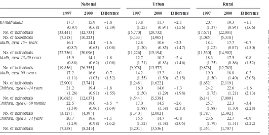
In our measures of poverty rates, we include all individuals found living in the interviewed households, whether or not the persons were selected to be interviewed individually (see the discussion of the selection process for individual interviews, in Chapter 2). We separately calculate headcount measures of poverty for children under age 15 and adults over 15. We break down children into age groups of 0–59 months and 5–14 years. We disaggregate adults into prime-aged, 15–59 and elderly, 60 and over. Standard errors are adjusted for clustering at the enumeration area.3

(45)

LEVELS OF POVERTY AND PER CAPITA EXPENDITURE

21

Percent of Individuals Living in Poverty: IFLS, 1997 and 2000

National Urban Rural

1997 2000 Difference 1997 2000 Difference 1997 2000 Difference

All individuals 17.7 15.9 –1.8 13.8 11.7 –2.1 20.4 19.3 –1.1

(0.97) (0.68) (1.19) (1.25) (0.94) (1.56) (1.37) (0.94) (1.66) No. of individuals [33,441] [42,733] [15,770] [20,732] [17,671] [22,001]

No. of households [7,518] [10,223] [3,433] [4,905] [4,085] [5,318]

Adults, aged 15+ years 16.1 14.4 –1.6 12.8 10.6 –2.3 18.4 17.7 –0.7

Adults, aged 15–59 years 15.9 14.1 –1.8 12.7 10.2 –2.4 18.3 17.5 –0.8

Adults, aged 60+years 17.2 16.6 –0.7 14.2 13.2 –1.0 19.0 18.8 –0.2

Ch_{ildren, aged 0–14 years} ₂₁_.₂ ₁₉_.₄ _–1_.₈ ₁₆_.₀ ₁₄_.₆ _–1_.₃ ₂₄_.₂ ₂₂_.₆ _–1_.₆

Ch_{ildren, aged 0–59 mont}h_s ₂₂_.₅ ₁₉_.₀ _–3_._{5 *} ₁₇_.₀ ₁₄_.₅ _–2_.₆ ₂₅_.₇ ₂₂_.₃ _–3_.₄

Ch_{ildren, aged 5–14 years} ₂₀_.₇ ₁₉_.₆ _–1_.₁ ₁₅_.₅ ₁₄_.₇ _–0_.₈ ₂₃_.₆ ₂₂_.₇ _–0_.₉

(46)

surprisingly, poverty rates for children are higher than for the aggregate population, since poorer households tend to have more children than do the non-poor. Also the adults in these households may be younger, with less labour market experience, also leading to lower incomes and pce. The difference in this case is large, 21% of all children and 23% of children under 5 years were poor in late 1997, as against 16% of prime-aged adults. Headcount rates for the elderly are not very different than rates for other adults, which may reflect a high degree of the elderly living with their adult children. In urban areas the poverty-rate differential between the elderly and prime-aged adults is slightly larger, which probably reflects that an elderly person is more likely to be living apart from their children if they live in an urban area. Headcount rates are higher in rural areas: 20.4% in rural areas for all individuals, as against 13.8% in urban areas in 1997.

What is perhaps surprising is that the headcount rate actually decreased slightly by late 2000, to 15.9% for all individuals, and to 19.4% for children. Neither decline is statistically significant at 10% or lower levels, although the decline for children under 5 years is at the 5% level. Measures of the poverty gap and squared poverty gap also show small, but not statistically significant, declines between 1997 and 2000 (see Tables 3.5a, b).5, 6_{Independent est}_i_{mates of poverty throughout the cr}_i_s_i_{s per}_i_{od show}

consistent findings. Using SUSENAS data and the same poverty lines that we use, Pradhan et al. (2001) and Alatas (2002) find that poverty rates climbed from 15.7% in February 1996 to 27.1% by February 1999, falling to 15.2% by February 2000.7

(47)

enormous importance that food prices, especially rice, play in determining levels of expenditure (see Alatas 2002, for a more formal simulation of this point). However, households are not passive in response to sharp changes in their environment, changes in behaviour are also greatly responsible for the recovery that has occurred.

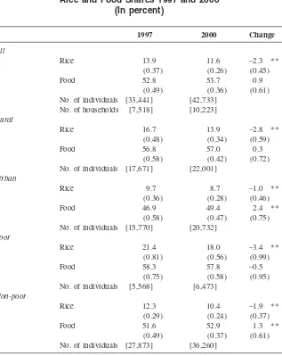
Table 3.2 demonstrates why rice prices can play an important role in changing real incomes, at least for consumers. Here we present budget shares of rice and all foods not including tobacco and alcohol (including consumption of foods grown at home). The mean food share barely changed over the entire sample, although it did rise for urban and non-poor individuals. On one level this could be interpreted as indicating a decline in welfare of these groups, although evidence on pce reported below belies this interpretation except for the very top of the distribution. The mean rice share was nearly 14% in 1997 and fell to 11.6% in 2000, a significant decline. Rice shares declined for all the groups we examined: urban and rural, poor and non-poor. The decline in rice shares evidently represents a behavioural change by households in their consumption patterns, plausibly in response to the relative rise in rice prices, although we don’t show that rigorously. The levels of rice share are especially high for the poor and in rural areas, 21% and 17% respectively. This underlines the importance of rice price as a determinant of well-being of the poor.

Of course for agricultural households, who both produce and consume rice, it is not the rice share of the budget, but the net demand of rice that is relevant to whether real incomes will decline or rise as the relative price of rice rises (Singh et al. 1986). Those rice farmers who are net sellers of rice will have favourable real income effects (all else equal) from a relative price increase. We do not have data in IFLS that can distinguish net sellers from net buyers. Many rice farmers will be net buyers of rice, especially if they own only a small amount of land, as most Indonesian farmers do. A study of income among farmers between 1995 and 1999 shows that larger landowners derive a larger fraction of their income from farming than do smallholders, who rely much more on non-farm income sources. Between 1995 and 1999, farmers, especially large farmers, experienced an

increasein income (Bresciani et al. 2002). To the extent that higher rice prices were capitalized into land prices, this differential effect by land size was enhanced. Hence the rapid changes in relative prices hit different parts of the population in different ways.

(48)

(49)

By comparing the years 1997 and 2000, as we do in this report, we propose to measure the medium-run measure of the impact of the crisis. However this may not provide the best medium-run measure of the impact. Rather one could compare the 2000 results with the level of poverty (or other dimensions of welfare) that would have been expected in 2000 had the crisis not occurred (for instance, Smith et al. 2002, analyse changes in wages and employment from 1993 to 1998 using this approach). This is difficult, requiring strong assumptions about what would have occurred over time, and certainly would require using data from pre-crisis years

can be compared to the 1997 poverty rates of all people who lived in the 1997 origin households. Poverty rates in 2000 in these split-off households poverty in 1997. We can conclude that split-off households do not occur randomly.Evidently there are forces which lead younger, better educated youth to leave their poor origin households, forming new households in which their real pceis subsequently higher (see Witoelar 2002, who tests whether these split-off and origin households should be treated as one extended household, rejecting that hypothesis). Clearly this pattern needs to be examined more closely in future work.

Means and medians of real per capita expenditure (pce), overall and by rural/urban residence, are reported in Table 3.4 for all individuals and the poor and non-poor separately. All values are deflated to December 2000 rupiah values and to Jakarta as the base region (see Appendix 3.A). As one can observe, median pces increased by a small amount, 4.5%, to just over Rp 200,000, but mean pces fell by roughly 11.5%, to Rp 292,000; a fall which is statistically significant at almost 5%. Among urban residents mean pce fell by nearly 20% (significant at 5%), compared to a 5.5% decrease (not significant at any standard level) among rural residents.

(50)

26

ANDARDS

TABLE 3.3

Percent of Individuals Living in Poverty for Those Who Live in Split-off Households in 2000: IFLS, 1997 and 2000

National Urban Rural

1997 2000 Difference 1997 2000 Difference 1997 2000 Difference

All individuals 21.4 12.7 –8.7 ** 16.3 8.7 –7.5 ** 24.9 16.2 –8.7 **

No. of households [1,545] [1,839] [714] [995] [831] [844]

Adults, aged 15+ years 19.3 11.5 –7.8 ** 14.8 7.9 –7.0 ** 22.8 14.9 –7.9 **

Adults, aged 15–59 years 19.3 11.1 –8.2 ** 15.0 8.0 –7.0 ** 22.7 14.1 –8.6 **

Adults, aged 60+years 19.1 16.8 –2.3 13.5 5.3 –8.3 ** 23.8 23.4 –0.4

(2.10) (2.74) (3.46) (2.32) (2.09) (3.12) (3.34) (3.97) (5.19)

No. of individuals [627] [326] [313] [139] [314] [187]

Ch_{ildren, aged 0–14 years} ₂₆_.₄ ₁₆_.₀ _–10_._{4 **} ₂₀_.₉ ₁₁_.₈ _–9_._{1 **} ₂₉_.₃ ₁₉_.₁ _–10_._{2 **}

(2.26) (1.71) (2.83) (3.13) (2.52) (4.02) (3.00) (2.35) (3.81) No. of individuals [2,525] [1,656] [1,015] [778] [1,510] [878]

Ch_{ildren, aged 0–59 mont}h_s ₂₉_.₇ ₁₄_.₈ _–14_._{8 **} _–14_.₈ ₉_.₆ _–15_._{3 **} ₃₂_.₃ ₁₈_.₉ _–13_._{4 **}

(2.81) (1.70) (3.28) (4.31) (2.43) (4.95) (3.68) (2.40) (4.39

No. of individuals [699] [859] [293] [406] [406] [453]

Ch_{ildren, aged 5–14 years} ₂₅_.₁ ₁₇_.₂ _–7_._{9 **} ₁₉_.₁ ₁₄_.₁ _–5_.₀ ₂₈_.₁ ₁₉_.₃ _–8_._{8 *}

(2.25) (2.31) (3.23) (2.97) (3.37) (4.49) (3.01) (3.16) (4.36)

No. of individuals [1,826] [797] [722] [372] [1,104] [425]

john strauss et al indonesian living standards before and after the financial crisis evidence from the indonesia family life survey

from฀

www.rand.org

฀as฀a฀public฀service฀of฀

the฀RAND฀Corporation.

6

Jump฀down฀to฀document

Purchase฀this฀document

Browse฀Books฀&฀Publications

Make฀a฀charitable฀contribution

Visit฀RAND฀at฀

www.rand.org

Explore฀

RAND฀Labor฀and฀Population

฀

View฀

document฀details

For฀More฀Information

Support฀RAND

Indonesian

Living Standards

Before and After the Financial Crisis

Contents

List of Figures

List of Tables

Acknowledgements

List of Authors

1

The Financial Crisis

in Indonesia

2

IFLS Description and

Representativeness

3

Levels of Poverty and

Per Capita Expenditure