®
Digital
Resources
Electronic Survey Report 2013-020
Lessons from a Dialect Survey
of Bena: Analysing Wordlists
Lessons from a Dialect Survey of Bena
Analysing Wordlists
Bernadette Mitterhofer
SIL International® 2013
SIL Electronic Survey Report 2013-020, October 2013
Lessons from a
Dialect Survey of Bena
Analysing Word Lists
Bernadette Mitterhofer
S1048686
University of Leiden
MA thesis paper
MA of African Linguistics
First reader: Thilo Schadeberg (University of Leiden)
TABLE OF CONTENTS
2.3.1 Linguistic Maps and Atlases... 11
2.3.2 The Comparative Method... 16
2.3.3 The Blair Method ... 18
2.3.4 Levenshtein Distance and Gabmap ... 20
3 THE SOCIOLINGUISTIC SURVEY OF THE BENA LANGUAGE... 24
3.1 THE BENA PEOPLE AND THE BENA LANGUAGE... 24
4 ANALYSIS OF THE BENA WORD LISTS... 35
4.1 INTRODUCTION... 35
4.2 ANALYSIS USING THE BLAIR METHOD AND LINGUISTIC MAPS... 35
4.2.1 Phonological Findings ... 36
4.2.2 Lexical Findings... 41
4.3 ANALYSIS USING GABMAP... 56
5 EVALUATION OF METHODS AND CONCLUSION... 64
5.1 LINGUISTIC MAPS... 64
5.2 BLAIR METHOD... 64
5.3 GABMAP... 65
FROM THE INTERNET... 75
FIGURES... 77
MAPS ... 78
TABLES... 80
1 INTRODUCTION
1.1
Motivation
In my work in Language Assessment with SIL in Tanzania the analysis and comparison of word lists is a quite frequent task. For this reason I started to look into different methods of
analysing word lists. The data collected during a sociolinguistic survey of the Bena1
language provided a good opportunity. Unlike after other surveys, we did not come back with a good general idea of the linguistic layout of the area, and the sociolinguistic data we collected was not very straightforward. The analysis of the linguistic data became even more important than before and a comparison of some of the methods used was needed.
When someone begins to learn a new language, he usually starts with words and some phrases to build up vocabulary before learning all the intricate rules of the language.
Likewise, linguists, especially those working on formerly “unknown”2 languages start with
the elicitation of a word list. For the analysis of a language, a word list is a good starting point and analysing word lists has always been a part of the work of linguists. One of the reasons for using word lists is that in order to understand one another, speakers have to recognise the words the other speakers are using, since “as long as the listener correctly recognises words, he will be able to piece the speaker’s message together” (Van Heuven 2008:43).
Thus word lists are an integral part of the data collection in any language. However, after the word lists have been collected, the question arises what methods can and should be employed in the analysis of the data. Depending on the research questions different
methods can be used. If the aim is to analyse the phonological3 system of a language, the
analysis will be to some degree different from an analysis that compares word lists of different languages or dialects in order to evaluate their relatedness.
1
1.2
Research Questions and Purpose
During a linguistic research a lot of data are collected. As data collection in itself is usually not the aim, the question arises how to analyse the data, and after analysis, how to present the results in a logical and clear way.
More specifically, what can be done with the data collected during the sociolinguistic survey of the Bena language in order to give a clear picture of the dialectal situation of the Bena language?
Concentrating on the data in the word lists, what methods can be used to analyse the data and what possibilities are there to present the results from these data?
How do these methods to analyse data and present linguistic results compare with each other?
Therefore, the purpose of this thesis is to look at the advantages and disadvantages of different methods of comparing and analysing data. In order to do this I took the data collected during the sociolinguistic survey of the Bena language and applied some of the methods to these data. The data are word lists which were collected to investigate the different dialects of the Bena language and their relationships with each other. Then I compared the results and the methods.
1.3
Thesis Overview
This chapter of introduction into the topic is followed by a chapter about dialectology where a definition of dialect versus language is given with a short historical overview of dialectology and the description of some methods of analysing and comparing dialects. The third chapter gives some background information on the Bena people of Tanzania and their language. It also describes the research questions of the dialect survey of the Bena language, what type of data and how the data were collected. The fourth chapter goes into the
2 COMPARING DIALECTS
2.1
Dialects
As the thesis is about a dialect survey and the comparison of the dialects of the Bena language, we need a definition of what constitutes a dialect. Usually, a dialect is seen as a language variety which signals a person’s background and origin, mainly geographically, but also socially or even occupationally.
Interestingly, even within linguistics there is no clear-cut definition of what constitutes a dialect or what a language. Rather, it depends on several factors which might contradict each other and usually, dialect is defined in opposition to language or other speech varieties (like jargon, etc.).
For a long time dialects were seen as corrupted versions of the standard language and the assumption was that they were lacking on all levels, especially in grammatical structures in comparison to the standard language. However, it has been established that this assumption of dialects as deficient variants of standard languages is false, although it is still a widely-held belief among the general population.
Dialect and standard language might also be differentiated by their different domains of use. Dialects are used more among family and friends, in local settings and work places and they are usually spoken, not written. The standard language is used in public and official domains, e.g. in education, administration, literature, science, etc. Yet, this is not always the case, as speakers of the speech variety which has become the standard language will use the standard language also in the domains of family and local settings. At the same time dialects sometimes are used also in more formal and official settings.
A similar approach in defining dialect and standard language is by their speakers: dialects are (seen to be) spoken by farmers, tradesmen, generally blue-collar workers and people with less education. The standard language is spoken by the middle and upper classes, government officials, civil servants, and generally people with higher education. Even so,
this dichotomy does not always hold true4 and seems to be rather a coincidence.
other, they would be considered to speak two separate languages. In other words, a dialect is a variant of another language variety (another dialect or a standard language) with enough similarities in the lexicon and the grammar to retain mutual intelligibility between the two systems. However, this criterion does not need to be applied strictly between a dialect of a language and the standard language. Even if dialect A differs from the standard language so much that speakers of dialect A and speakers of the standard language do not understand each other, dialect A will still be considered a dialect of this standard language if there is a dialect B which is understood both by speakers of dialect A and speakers of the standard language (and speakers of dialect B understand both dialect A and the standard
language).5
Another (cultural) criterion is the opinion of the speakers about their form of language. If speakers think of their language variety as a variation of a more standard form of language or an already standardised form of the language is perceived as norm, they would be considered to speak a dialect.
The criterion of geographical area is probably the criterion which is most widely used and implied. Usually, when someone speaks of a dialect they mean a speech variety which is spoken in a certain area that is not too large. In contrast, a language is a speech variety which is spoken more widely and in several areas. There are usually more people who speak the (standard) language than the dialect and the geographical range of possible communication is larger for a language than a dialect. Often dialectology is used to mean dialect geography, where different features of dialects are put on a map. Although this is how dialectology began and still is an important way of presenting data, it is only one branch of dialectology. Nevertheless, it shows the importance of the criterion of geographical area in the definition of language and dialect.
The political status of a language variety is another important factor for the differentiation between dialect and language. Linguistically very similar language varieties where the speakers understand each other without problems are sometimes called different languages due to political borders. For example, speakers of Dutch dialects and speakers of German dialects on the Dutch/German border have no difficulty understanding each other.
Linguistically, these German dialects are more similar to the Dutch dialects than to German dialects which are spoken in a greater distance. On the other hand, linguistically very different language varieties without any mutual intelligibility can sometimes be called dialects for political and usually also social reasons, i.e. because they are spoken within a
5
single political entity, e.g. the ‘dialects’ of Chinese within the territory of the People's Republic of China. (Löffler 2003; Chambers and Trudgill 1998; Dialect 2011; Vajda, 2001)
One thing seems to be clear: The term dialect always infers relatedness. A language variety
cannot be called a dialect without defining which of the other language varieties it is related to or which language it is a dialect of. (Möhlig 1981:451) Chambers and Trudgill state that there is truth in the claim that ‘a language is a dialect with an army and a navy’ because it “stresses the political factors that lie behind linguistic autonomy”. (1998:12)
In this thesis, I use the term dialect according to the definition of the Ethnologue. The Ethnologue (Lewis 2009; emphasis in original) defines language and dialect as follows:
[e]very language is characterized by variation within the speech community that uses it. Those varieties, in turn, are more or less divergent from one another. These divergent varieties are often referred to as dialects. They may be distinct enough to be considered separate languages or sufficiently similar to be considered merely characteristic of a particular geographic region or social grouping within the speech community. Often speakers may be very aware of dialect variation and be able to label a particular dialect with a name. In other cases, the variation may be largely unnoticed or overlooked. Not all scholars share the same set of criteria for distinguishing a “language” from a “dialect”. Since the fifteenth edition,
Ethnologue has followed the ISO 639-3 inventory of identified languages as the basis for our listing. That standard applies the following basic criteria for defining a language in relation to varieties which may be considered dialects:
Two related varieties are normally considered varieties of the same language if speakers of each variety have inherent understanding of the other variety at a functional level (that is, can understand based on knowledge of their own variety without needing to learn the other variety).
Where spoken intelligibility between varieties is marginal, the existence of a common literature or of a common ethnolinguistic identity with a central variety that both understand can be a strong indicator that they should nevertheless be considered varieties of the same language.
Where there is enough intelligibility between varieties to enable communication, the existence of well-established distinct ethnolinguistic identities can be a strong indicator that they should nevertheless be considered to be different languages.
These criteria make it clear that the identification of “a language” is not solely within the realm of linguistics.
In this definition the focus lies mainly on the linguistic side of the definition, namely
intelligibility between speech varieties/dialects. Since the focus of this thesis is on analysing word lists, it is the most suitable definition for this purpose.
gender, social network, education and trade. Dialectology is one of the oldest branches of linguistics. It focuses on the geographic distribution of language variation (dialects) within a language.
People have always noticed the differences between the different dialects and sometimes remarked on them in letters and travel diaries. Even so, it took the scientific world some time to become interested in them and find that “dialects are a valuable source of
information about popular culture. They reflect not only the history of a language but, to a great extent, the ethnic, cultural, and even political history of a people as well.” (linguistics (2011), Encyclopædia Britannica) The oldest known attempts to investigate dialect divisions in a more scholarly way dates from 1821. Both Coquebert de Montbret in France and J. A. Schmeller in Germany published a dialect map independently of each other. (Heeringa 2004:9)
Still, until the second half of the nineteenth century, linguists mainly worked on and studied written texts in order to establish the relationships between the languages of the world. This was done by searching for rules which would show the phonetic
correspondences between words of these languages.
Through the study of classical languages, their interest in the historical development of languages, and their discovery of the relationships between many modern and classical languages, a German school of linguists called the Neogrammarians were the first to begin the search for general principles which would apply to all language change. This led them
to propose their famous hypothesis of the Ausnahmslosigkeit der Lautgesetze, or
‘exceptionlessness of sound changes’. This meant that sound changes are regular and follow rules and do not happen totally at random.
The hypothesis that sound laws are exceptionless turned out to be false, especially as it did not take into account the social character of language and the influence of cultural aspects on sound changes. In spite of that, it is a good working hypothesis, and it sparked an increased interest of many linguists in dialects. Dialects were seen as a source which would help in the determination of older and more regular forms of words and structures than the standard languages. This again would lead to the identification of sound changes and also the reconstruction of an older form of the language.
Another impetus to investigate dialects came from the Romantic view of regional speech forms as part of folklore and tradition. There was also the feeling that due to modernisation and urbanisation these rural speech forms were rapidly declining and becoming extinct.
first to undertake a dialect survey on a large scale was Georg Wenker, a German school teacher in 1876. He set up a questionnaire of 40 sentences written in Standard German which would display certain linguistic features. These he sent to every village in Germany which had a school and asked the local headmaster or head teacher to rephrase every sentence in the local dialect. About 45 000 questionnaires were filled out and returned. (Chambers and Trudgill 1998:15)
Due to the wealth of data Wenker had to limit his analysis to the variants of certain words within a certain area of Germany in order to make his findings accessible. In 1881 the first linguistic atlases were published, consisting of maps, with each map charting a single feature according to its geographic distribution. (Chambers and Trudgill 1998:16) This work was continued by Wenker and other linguists, and between the years 1926 and 1956 the volumes of the ‘Sprachatlas des Deutschen Reiches’ were published. (Löffler 2003:25) Similar projects were undertaken in other countries.
However, the use of postal questionnaires in data collection was soon abandoned. The first survey to use trained fieldworkers was the linguistic survey of France which began in 1896. Jules Gilliéron wanted to improve Wenker’s method and devised a questionnaire with specific items for which responses could easily be elicited. Then he trained Edmond Edmond in the use of phonetic notation. From 1896 to 1900, Edmond cycled through France conducting interviews and recording the responses. As Edmond sent his results periodically back to Gilliéron, analysis and the publication of the results began almost immediately. The final volume was published in 1910. (Chambers and Trudgill 1998:17)
Due to the quality of the results and effectiveness of Gilliéron’s French survey in which he used a phonetic transcription to elicit data proved to be highly influential. Since then, many trained linguists have followed this method in many other countries around the whole world.
2.3
Methods for Comparing and Analysing Dialects
There are a number of ways to compare languages, dialects or other speech varieties. Among other things, the type of analysis depends on the following:
• The purpose of the research and the research questions,
• The parts of the language system which are compared (e.g. phonology6, lexicon,
• The type of data (e.g. word lists, single sentences, stories, written texts, recordings, etc.).
The following are descriptions of some methods on how to analyse and compare dialects, together with their purpose. Some methods have been in use for centuries, some only in more recent years - with new technology also come new methods of analysis and of
presentation. A good overview and descriptions of other methods can be found in Heeringa 2009 chapter 2.
2.3.1 Linguistic Maps and Atlases
Languages do not occupy certain spaces or geographic areas in themselves, rather it is the speakers of languages who live in certain areas. It is in this sense that linguistic atlases are a means of displaying the distribution of languages and dialects with their respective borders in the areas where they are spoken. The following map (Map 1) shows the different
languages spoken in Tanzania.
Map 1 – Language map of Tanzania (Lewis 2009).
analyse and show results of the comparison of different features between dialects e.g. the distribution of certain sounds, different words with the same meaning, etc.
There are different ways to represent these variations within language: Two classic ways are
by drawing isoglosses7 between the language features in question or by placing a symbol at
each research location representing a certain variation of the feature in question.
The map below (Map 2) gives an example of lexical isoglosses that split Germany in three major areas.
The next map (Map 3) is taken from the Atlas zur deutschen Alltagssprache8. It shows the
variation in pronunciation of the word das (the, neuter) in Germany, Austria and
Switzerland9. Different coloured markings of various shapes give the locations where certain
pronunciations were reported.
Map 3 – The distribution of the variations in pronunciation of the German neuter article das in Germany, Austria and Switzerland (Atlas zur deutschen Alltagssprache (AdA)).
Linguistic maps which show the distribution of languages have also been used in African linguistics since the beginning. But the vastness of the continent and the number of
languages spoken made it difficult to be as comprehensive as in the study of the languages of Europe. Hence, the use of linguistic atlases as a means of analysing language varieties started only in the last century.
One of the first attempts was a dialect map of the Nyamwesi language area in 1910 by B. Struck .(Möhlig 1981:448) Towards the end of the 1930s E. Boelaert, following in Georg Wenker’s footsteps, undertook a dialect survey using questionnaires in Belgian Congo. This
8
The Atlas zur deutschen Alltagssprache (‘Atlas of German everyday speech’) is a project which was started in 2002 and aims at capturing the diversity of German by collecting regional variants of lexical items along with different pronunciations and some grammatical forms using an online questionnaire.
9
was followed by studies both in the field of historical linguistics and in the field socio-linguistics and resulted in 1948 and 1950 in linguistic maps of that area. (G. van Bulck
1948, G.Hulstaert 1950 in Möhlig 1981:449) Even in Malcom Guthrie’s The Classification of
the Bantu Languages (1948) the geographical aspect plays a major role.
The following two maps (Map 4 and Map 5) are from a pilot study in 1969 for a language and dialect atlas of Kenya. Both show the different terms for ‘leopard’ in the mountain dialects on the east side of Mount Kenya. (Möhlig 1981:458f.) Map 4 shows the different terms as symbols according to their distribution by location; Map 5 shows the distribution of these terms with the help of isoglosses.
Map 5 – The distribution of the different terms for ‘leopard’ with the help of isoglosses (Möhlig
1981:459).
The advantage of language maps is that they show the geographical distribution of
language varieties or certain linguistic features in a concise and easily comprehensible way.
2.3.2 The Comparative Method
The Comparative Method is a technique for comparing languages in order to confirm or refute hypothesized relationships between these languages. In the case of their relatedness it
aims to reconstruct a proto-language10.
The idea of having a method to demonstrate relatedness of languages and to find proto-languages dates back to the seventeenth century, when Marcus van Boxhorn proposed an Indo-European proto-language, where all the Germanic, Romance, Celtic, Baltic, Persian, Slavic, Greek and Sanskrit languages derived from. He also described a methodology for comparing the languages and proving their relatedness.
The Comparative Method itself was developed during the nineteenth century with key contributions from Rasmus Rask and Karl Verner, two Danish scholars, and Jacob Grimm, a German scholar. August Schleicher was the first linguist to publish reconstructed forms from a proto-language in 1861. Key to the method is the Neogrammarian Hypothesis of the ‘exceptionlessness of sound laws’, as the method assumes regular correspondences between
sounds11 in related languages. This is only the case if sound changes from the
proto-language followed regular patterns.
In this method one starts with making list of words which are likely to be cognate words12
from the languages that are compared. One compares the words feature by feature and if there is a regularly recurring match between certain sounds or sequences of sounds in the words (of similar meanings) they are probably related.
The next step is to establish regular sound correspondences. Phonetic similarity13 in itself is
not enough, because this could be the result of borrowing or chance. The sound
correspondences have to be recurring like for example t- and z- in English and German:
English: ten two tongue tooth toe
German: zehn zwei Zunge Zahn Zeh
10
A proto-language is a language which is the “common ancestor”, e.g. from which the compared languages can be derived.
11
Step three comprises of reviewing these correspondence sets and separating the sound
changes which are independent of their environment14, called unconditioned sound
changes, from conditioned sound changes, where the sound changes only took place in certain contexts (e.g. after [a] but not after another vowel).
For instance, the following table (Table 1) shows an example within the Romance language family which their common ancestor Latin.
Gloss body raw chain to hunt
Italian corpo crudo catena cacciare
Spanish cuerpo crudo cadena cazar
Portuguese corpo cru cadeia caçar
French corps cru chaîne chasser
Table 1 – Sound correspondence sets in the Romance language family.
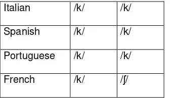
If we look at the sound of the first consonant in each word in Table 1 we find two correspondence sets: /k/ with /k/ and /k/ with /ʃ/ (see Table 2).
Italian /k/ /k/
Spanish /k/ /k/
Portuguese /k/ /k/
French /k/ /ʃ/
Table 2 – Sound correspondences in the Romance language family.
/ʃ/ in French only occurs before /a/ (where all the other languages also have /a/) and /k/ occurs before all other vowels. Consequently, it is the environment that conditions the difference in the correspondence sets and they all derive from the proto-sound /k/ (spelled <c> in the other languages and Latin the proto-language).
The next step then is to reconstruct the proto-sounds for each sound correspondence set. This is done with the help of typology and the knowledge of which sound changes are more likely than others, e.g. the voicing of voiceless plosives (i.e. [t], [p], [k], etc.) between vowels is much more likely than voiced plosives (i.e. [d],[b],[g], etc.) to become devoiced.
The last step is the examination of the reconstructed sound system for symmetry and likelihood.
14
There are of course also problems with this method. For one, the underlying assumption that “sound laws have no exceptions” is not always true, as there are several types of change that cause words to alter in non-regular ways (e.g. by analogy).
Borrowed words if not recognised as borrowed can skew the data. Borrowings can occur on a larger scale; certain features in the sound system, the grammar or the lexicon can be adopted by a number of (unrelated) languages in a geographical area. This is called areal diffusion and could lead to the reconstruction of a false proto-language.
Another danger lies in the subjectivity of the reconstruction in the case of unknown proto-languages, as there is no evidence for the actual proto-sounds which are reconstructed. Loanwords from the proposed proto-language into another (unrelated) language can help to verify some of these sounds. For further details about the Comparative Method see
Campbell, 2004.
2.3.3 The Blair Method
This method for comparing word lists has been developed in South Asia by Language Survey Teams of SIL. It is a lexicostatistical method somewhere between simple inspection and the Comparative Method.
It follows the first three steps of the Comparative Method by aligning words with similar meanings and looking for sound correspondences. If certain correspondences occur at least three times in a 200-item word list they are considered as regular sound correspondences. Like in the Comparative Method, one determines whether these correspondences are conditioned sound changes or whether they are independent of their environment. The correspondences and the words where they can be found are documented.
However, instead of reconstructing the proto-sounds for each of the sound correspondences as one does with the Comparative method, the next step is to judge the phonetic similarity
of words. The corresponding segments15 in a pair of words are analysed and placed in one
of three categories (Blair 1990):
Category 1
Exact matches (e.g., [b] occurs in the same position in each word.)
Phonetically similar segments which occur consistently in the same position in three or more word pairs. For example, the [g]/[gɦ] correspondences in the following entries from these two dialects would be considered category one:
Gloss Dialect 1 Dialect 2
Consonant segments which are not correspondingly similar in a certain number of pairs. [...]
Vowels which differ by two or more phonological features (e.g., [a] and [u]).
Category 3
All corresponding segments which are not phonetically similar.
A segment which corresponds to nothing in the second word of the pair. For example, the [l]/[#]16 correspondence in the word for boy in the example above.
If at least half of the segments compared are in Category 1 and at least 75% of the segments compared are in Category 1 and Category 2 the compared words are judged to be
phonetically similar.
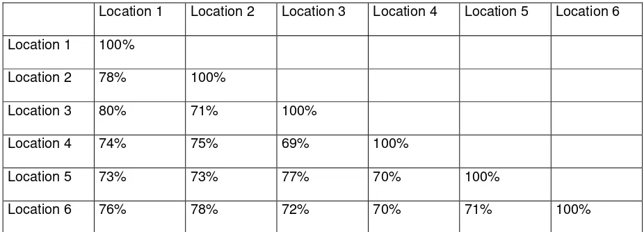
These phonetically similar items of the word list can then be presented in different ways. For example, they can be shown in the form of maps and linguistic atlases as described in Section 2.3.1 (p. 11); or they can also be tabulated and the percentage of similar glosses between each two word lists calculated and put into a matrix like the following in Table 3.
16
Location 1 Location 2 Location 3 Location 4 Location 5 Location 6
Table 3 – Example of a similarity matrix showing the percentage of items similar between each pair of
locations.
This matrix shows that, if we follow the column of Location 1, there are 78% similar glosses of all the items elicited between Location 1 and Location 2, 80% similar glosses of all the items elicited between Location 1 and Location 3, etc.
Unlike the Comparative Method, the Blair Method does not try to prove the relatedness of languages (although it starts with the same steps) but rather investigates intelligibility between languages. The more words of one variety are similar to another, the likelier it is that speakers of these varieties will recognise these words and understand each other. For this reason borrowings and areal diffusion do not pose a big problem.
2.3.4 Levenshtein Distance and Gabmap
Levenshtein Distance
The Levenshtein distance17, also called String (Edit) Distance, is a metric which measures
distance or dissimilarity (and therefore also similarity) between two text strings. The
Levenshtein distance d(s1,s2) is the minimum number of operations (insertion, deletion and
substitution) needed to change one string s1 (or word) into anotherstring s2. The greater the
Levenshtein distance, the more different the strings (or words) are.
For example, the Levenshtein distance between the words Baum ‘tree’ and Blume ‘flower’ is
2. Aligning the two words, we substitute a to l and then add e.
B a u m
B l u m e
Two operations (substitution and insertion) are needed to transform the word Baum into
Blume.
Levenshtein distance is used, for instance, in spell checking, DNA analysis, speech recognition, etc. In dialectometry, it measures the minimum number of operations
transforming one gloss (and its pronunciation) of a word from one location (or informant) into the corresponding gloss from another location (or informant).
Levenshtein distance was first used by Kessler (1995) in measuring dialect pronunciation differences in Irish. Heeringa (2004) in his dissertation successfully applied it in measuring Dutch dialects and Norwegian dialects. It has also been effectively applied in comparing English speech variants in England and the USA (Nerbonne 2005), and Bulgarian dialects (Osenova et al. 2007). Yang (2009) applied it to Nisu, a Burmic language in China and has
shown that it is also possible to adapt Levenshtein distance to use it in comparing tonal18,
isolating19 languages. She and Castro also investigated the best representation of (contour)
tone in the Levenshtein distance algorithm in relation to intelligibility (Yang et al. 2008).
By comparing the Levenshtein distances of Norwegian dialects with native speakers’
perceptions of these dialect differences, Gooskens and Heeringa (2004:203) found that they correlate (r = 0.67, p < 0.001), which would make Levenshtein distance a good
approximation of perceptual distances between dialects. For Scandinavian languages Gooskens (2006:111) found a strong negative correlation (r = - 0.82, p < 0.01) of Levenshtein distance with intelligibility test results. This means that the greater the
linguistic distance between dialects, the more difficult it will be to understand each other.20
Levenshtein distance counters the main weakness of traditional dialectological methods (linguistic atlases, the comparative method): subjectivity. It measures the aggregate differences of all available data, giving the overall linguistic distance between language varieties and providing an objective measure.
18
Tone refers to the use of the pitch or register of the voice as a means to differentiate between words that are otherwise identical. Unlike intonation, each syllable carries its own tone and the difference in tone alone can change the meaning of the word, either lexically or grammatically. East Asian languages are most widely known as examples of tonal languages, but most Bantu languages (Africa) are also tonal languages.
19
An isolating language is a language where (most) words consist of a single morpheme (the smallest unit in a language which carries meaning). The opposite are synthetic languages where words are (usually) composed of at least two morphemes, e.g. the English word girl consist of only one morpheme, the German equivalent Mädchen has two morphemes: Mäd- ‘girl’ and -chen
20
Yet, it is a quantitative measure which correlates well with perceived differences and intelligibility between dialects. It does not measure (historical) relatedness between speech varieties.
Gabmap
Gabmap is a web application which has been developed to help dialectologists make mappings and statistical analyses of dialect data by providing easy-to-use dialect analysis tools. It has default settings for its analysing techniques for inexperienced users based on the experience of the authors, and features to help with checking results, e.g. multi-dimensional scaling for checking clustering results.
After uploading linguistic data21 and maps to Gabmap, the data is processed with
Levenshtein distance. The defaults for the Levenshtein distance were set to a variant which uses tokenised transcription, in which consonants and vowels are always kept distinct, but in which segments are otherwise only the same or different. All operations (insertion,
deletions, and substitutions) have the same weight (or cost). Word length is normalised22, in
order to not give greater weight to longer words. Based on the Levenshtein distances between all pairs of items the mean Levenshtein distance is calculated for each pair of varieties. (Nerbonne et al. 2011)
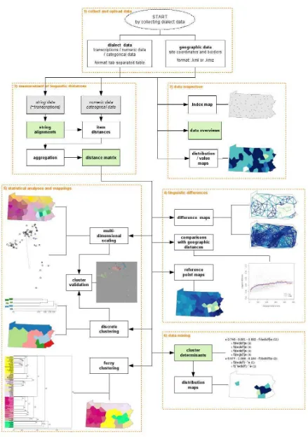
Besides generating data overviews, Gabmap produces a distance matrix. These distances are then projected onto maps and graphs and can be further explored with the help of
dendrograms (discrete and fuzzy clustering dendrograms), multi-dimensional-scaling, (dialect) distribution maps, and data mining for those features that determine certain clusters. (See Figure 1 below.)
3 THE SOCIOLINGUISTIC SURVEY OF THE BENA LANGUAGE
In September 2009 I was part of a team of SIL International which conducted a
sociolinguistic survey among the Bena people of Tanzania. The goal of this survey was to clarify questions about the dialectal situation of the Bena language.
3.1
The Bena People and the Bena language
The Bena people are one of the bigger tribal groups of Tanzania with about 670 000 people according to the Ethnologue (Lewis 2009). The Bena people are agriculturalists who
cultivate potatoes, wheat, rye, maize and other cold-resistant crops. The majority of the
Bena people live on a high plateau in the Njombe District23 of the Iringa Region in the
southwest of Tanzania, which is seen as the traditional Bena area. A small minority live on the plain in the Kilombero district in Morogoro Region. The two areas are separated by an uninhabited broken escarpment which is difficult to cross by foot and impassable by car. The language groups surrounding the Bena people are the Vwanji and the Kinga in the west, the Hehe and the Sangu in the north, the Ndamba and the Ngoni in the east, and the
Ndendeule, the Ngoni and the Pangwa in the south.
Map 7 – Bena language area and surrounding language groups (© SIL International 2006).
The Bena language (ISO bez) belongs to the Bantu languages24. The Ethnologue (Lewis
2009) classifies the Bena language as: Niger-Congo, Atlantic-Congo, Volta-Congo, Benue-Congo, Bantoid, southern, Narrow Bantu, Central, G, Bena-Kinga (G.60). Its lexical similarity is 71% with Pangwa [pbr], 65% with Hehe [heh], 55% with Sangu [sbp], 53% with Kinga [zga], 51% with Vwanji [wbi], 47% with Kisi [kiz]. Other names are: Ekibena or Kibena.
There are several different varieties of the Bena language. Most Bena speakers are aware of dialectal variation and usually seem to divide the Bena area into three to five dialect areas. Some older Bena people associate dialects with historic clans (but usually only if asked to name dialects).
24
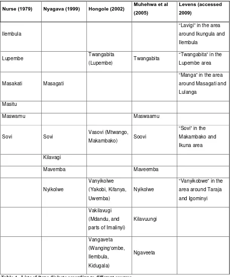
Table 4 below shows lists of dialects according to different sources in the literature.
Nurse (1979) Nyagava (1999) Hongole (2002) Muhehwa et al (2005)
Sovi Sovi Vasovi (Mtwango,
Makambako) Soovi
Table 4 - Lists of Bena dialects according to different sources
According to the Bena people25 the heartland of the Bena language is somewhere between
Mdandu and Njombe, but there doesn’t seem to be one variety of Bena that is considered a more superior or purer variety than the others.
Since Tanzania’s independence in 1961 the importance and prominence of Swahili (the national language of Tanzania) has increased greatly. Due to the fact that Swahili is the language in primary education, administration, business and trade, it is having a significant impact on the Bena language and, like most of the languages in Tanzania, the Bena
language is threatened by Swahili even though it is spoken by over half a million people.
There is some literature on the Bena language: mainly some short word lists26 and (sketch)
grammars, the most recent being Michelle Morrison’s dissertation A Reference Grammar of
Bena (2010).
3.2
Research Questions of the Sociolinguistic Survey of the Bena Language
The primary Research questions were:
Linguistic Differences
What are the regular phonological differences between the Bena varieties and how are they distributed, geographically and socially?
What are there regular morphophonemic or grammatical differences between the Bena varieties and how are they distributed, geographically and socially?
Where are different lexical items used and how significant are these differences?
Language/Dialect Relationships
How many varieties of the Bena language are there?
What is the central location for each of the Bena varieties and which is considered the “best” or “standard” variety?
What are the perceived differences between speech varieties?
What is the perceived comprehension between speech varieties?
25
These questions are part of our questionnaire for the group interview. (See Group Interviews, p. 31)
26
Where are the boundaries between the different varieties?
How big is the influence of Swahili and neighbouring languages?
Are there other factors that might influence the readability and intelligibility of produced literature in the Bena language?
Intelligibility and Readability of Finished Translations
Where was the Bena language of the texts perceived to be from?
What was the perceived quality of the Bena language of the texts?
How well did people understand the texts?
How well were people able to read the proposed orthography?
3.3
Procedure and Methods of Data Collection during the Survey
We started our survey by obtaining permission from the Commissioner of the Iringa Region and the Commissioner of the Njombe District to conduct our research and to gather
information about the Bena language. With their permission, we visited the different wards of the Njombe district. After the interviews with the ward leaders (see Ward Leader
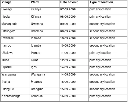
Interviews p. 31), we determined to conduct research in thirteen villages. Six villages were chosen for primary research and seven for secondary research. The only difference between primary and secondary research consisted in the word lists: in primary research locations a 301-item word list was taken, in secondary research locations a 94-item word list was taken. One factor in choosing villages for research was how pure and representative of the respective speech varieties the Bena people considered the language spoken in these villages to be. Other factors were a high percentage of Bena speakers in the village and geographic distribution.
Village Ward Date of visit Type of location
Liwengi Kifanya 07.09.2009 primary location
Itipula Kifanya 08.09.2009 primary location
Makanjaula Uwemba 09.09.2009 secondary location
Utalingoro Uwemba 09.09.2009 secondary location
Lwanzali Idamba 10.09.2009 secondary location
Itambo Idamba 10.09.2009 secondary location
Ukalawa Ikondo 11.09.2009 primary location
Ikuna Ikuna 12.09.2009 primary location
Ujindile Igosi 14.09.2009 primary location
Wangama Wangama 14.09.2009 secondary location
Ihanja Mdandu 15.09.2009 secondary location
Utengule Utengule 15.09.2009 secondary location
Kanamalenga Ilembula 16.09.2009 primary location
Map 8 – Bena language area with research locations in green capital letters (© SIL International 2010).
The Methods used to collect the data included the following:
Sociolinguistic Interviews
Word lists
Phrase Lists
Intelligibility Tests
Orthography Tests
3.3.1 Sociolinguistic Interviews
Ward Leader Interviews
We conducted an interview with ward leaders in eleven wards. The questions asked about the ethnic constituency, education, religious affiliation, and relationships between language varieties within the ward and with language varieties in other wards. This information helped to form a picture of the population demographics, the distribution of the language varieties and to decide which villages to choose as research locations.
Group Interviews
The village leader in each location was asked to assemble a group of at least 12 people - young, old, men, and women - who considered themselves to belong to the Bena people and who would be willing to participate in a group interview about the Bena language. In Utalingoro, Ikuna and Ujindile there were only 11 people participating. Conversely, in Kanamalenga a group of 54 formed. A total of 281 people took part in the interviews.
The people were asked a series of questions about the Bena area, their attitudes concerning the Bena language and Swahili, their way of speaking and their perception of other
varieties. We took detailed notes of the answers given, also noting any discussions or side-comments.
Religious Leader Interviews
Whenever possible, interviews were conducted with any Christian leaders present. The aim was to find out the language use in their religious services and what impact they thought a Bible in the Bena language would have on their ministry. In total, 13 religious leaders in ten villages were interviewed.
Teacher Interviews
If available, teachers were interviewed for information concerning school demographics and language use in schools. Seven teachers, each in a different village, were interviewed.
3.3.2 Word lists
people participating in the word list had been born in that village and had not spent significant time travelling or living elsewhere.
In every group the criteria of having men and women participants was met. However, the criteria of age proved to be a different matter. In each group there was at least one of the participants older than 50 years of age, usually two or three of five participants were older than 50 years of age. In three villages one of the participants was younger than 30 years of age. The youngest participant was 25 years old, the oldest two participants were 79 years old. In total, sixty-two Bena speakers took part in the elicitation of the word lists.
The word lists used consist of 301 items and 94 items respectively. 40 items were part of both word lists and were elicited in all thirteen locations. The elicited words are a mixture of nouns, verbs, numbers, adjective and interrogatives. To avoid synonyms, the Swahili equivalent of the Bena word was given with clarification words if needed. Verbs were elicited in the present progressive (third person singular) and imperative forms. In some cases the perfect form was used because it was more natural to elicit from Swahili.
Each word was transcribed using the International Phonetic Alphabet (IPA). Any discussion about word choice was noted on the elicitation form and although consensus in the word choice was sought, synonyms were written down as well. Afterwards, the word lists were recorded as spoken by one of the participants. Two linguists alternated in eliciting the word lists: one usually elicited the longer word list, the other usually elicited the shorter word list.
Our team also wanted to find out the speaker’s intuition — that is, how speakers of that speech variety would write words in their language. For this reason, during the elicitation of the word lists one of the participants was asked to write down the Bena glosses using the Swahili alphabet.
As each word list was taken, participants were asked about words that were different which had been elicited from previous word lists. The reason of this was to help clarify whether different words elicited in other locations were indeed words specific to that location or if they were synonyms or borrowed words.
3.3.3 Phrase Lists
convey the phrases we wanted to elicit. The phrases were written using the proposed Bena
orthography with some additions27 and afterwards recorded by one of the Bena speakers.
3.3.4 Intelligibility Tests
From newly translated parts of the Bible into the Bena language, a short text was chosen that would be easy to retell. In each location, we asked that someone from the group of Bena speakers, who could read well in Swahili, would read the text to the rest of the group. This was done to eliminate the problem of different pronunciations in dialects as the
reader’s pronunciation of words would match the group’s pronunciation of their dialect.
After the reading, each group was asked their opinion about the quality of the Bena
language used and where they thought the language of the text was spoken. They were also asked how much they understood from the text.
Then, to test their understanding, the people in the group were asked to retell the story. Except in the case of very detailed retelling, questions about some of the details of the story were asked specifically to test how much the people understood the text in depth.
The reading itself was recorded and all the responses were written down. This test was done in each location.
3.3.5 Orthography Tests
For this test, another text in the Bena language from the newly translated Bible parts and a second similar text in Swahili were chosen. In each location, the team asked for Bena speakers who could read Swahili and would be willing to try reading in the Bena language.
For each test, the person tested was asked to read the Swahili text first and a note was taken as to their general reading ability. Then they were given the Bena text to read. Each time when there appeared to be a problem with a word this was noted on a separate paper and the reading itself was recorded for later reference.
After the reading, each individual was asked his or her opinion about the quality of the Bena language used in the text and where they thought the language of the text was spoken. They were also asked how much they understood from the text, how difficult it was to read
and what they thought their difficulties in reading were. Another question was whether they had read anything in the Bena language or another local language before.
4 ANALYSIS OF THE BENA WORD LISTS
4.1
Introduction
Although we collected a lot of different data during the sociolinguistic survey of the Bena language, I am concentrating only on the data of the word lists which were elicited. The word lists were analysed in two ways:
First, the Blair Method (see section 2.3.3, p. 18), the more ‘traditional’ method of
comparing the glosses given in each village for the items of the word lists was applied. As it is part of the Blair Method to search for sound correspondences in order to make judgments about the similarity of glosses, it yields results both at the phonological and the lexical level. The results of the phonological analysis are presented in a table and in form of linguistic maps. The results of the analysis of lexical similarity are given in form of
matrices28 and some maps of a few items from the word lists are also given as examples.
Second, the data in the word lists together with a map of the area was uploaded to Gabmap which uses Levenshtein distance (see section 2.3.4, p. 20). This yielded difference matrices, dendrograms, multi-dimensional scaling plots and a number of maps.
In this section the analysis of the word lists from the thirteen locations in the Bena language area is presented. It starts with the results of the Blair Method, first the phonological
findings, then the lexical findings. Then follow the results using Gabmap.
4.2
Analysis using the Blair Method and Linguistic Maps
I chose to use the Blair Method rather than the Comparative Method, mainly because the glosses in the word lists are of varieties of the same language and the similarity and intelligibility between these varieties of today are under investigation, not the historical relationships and developments. Another reason for choosing the Blair Method is the comparability with the results using Levenshtein distance, which correlates with intelligibility rather than historical relationships.
I applied the following rules to judge the similarity29 between glosses of an item: If glosses
only differed in aspects of vowel quality (+/-ATR and length) they were counted as similar in the analysis. If the difference between glosses was their noun class prefix or verb tense marker they were also counted as similar. If a noun class prefix or verb tense marker appeared to be influencing the root of a gloss, the root was still considered a similar gloss.
28
Matrices were calculated with Excel.
29
Thus glosses like [ntsuːxi] and [ntsuki] ‘bee’ or [libaːnsi] and [libandi] ‘bark (of tree)’ are seen as similar, whereas [libaːnsi] and [likoːna] ‘bark (of tree)’ are not counted similar. If in a location for one item two glosses instead of one were given the item was counted twice, first with the first gloss in that location and the single glosses in the other locations and the second time with the second gloss in that location and the single glosses in the other
locations again. For instance, in Itipula we elicited [soːka] and [ŋgiːnda] for ‘axe’. So the item ‘axe’ was counted twice, first with [soːka] for Itipula and then with [ŋgiːnda] for
Itipula, whereas the glosses for ‘axe’ remained the same for the other locations. Tone30 was
noted in the word lists but not taken into account for this analysis.
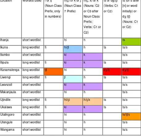
4.2.1 Phonological Findings
For the phonological comparison, I aligned the glosses of the different locations for each
item (word) and looked for corresponding phonemes31. I noted corresponding phonemes
Location Wordlist used f or tʃ
Table 6 – Phonological differences between the research locations
In the villages where the full word list (301 items) was elicited, numbers from one to ten were also asked. The consonant of the noun class prefix used was [f] in five of the six villages. In Kanamalenga it was [tʃ]. Map 11 below shows the distribution geographically.
Map 11 – The occurrence of [tʃi] and [fi] according to locations.
When all phonological differences are put together on a map, some isoglosses emerge: a group of four locations in the east and one distinctive location in the northwest. Four other locations show some phonological differences from the rest. (See Map 14 below)
Map 14 – All phonological differences according to locations.
4.2.2 Lexical Findings
For a lexical comparison, I compared glosses in a number of ways. Both identical and then
similar glosses32 were counted and the percentages between the glosses calculated according
to the number of items given in each pair of location.33
It should be noted that 3 of the 40 items which were elicited in all the locations, namely [liːho] ‘eye’, [likaːŋa] ‘egg’ and [seːŋga] ‘cow’, have identical glosses across all the speech varieties given in the thirteen locations. Two of the 94 items of the short word list which
32
Identical glosses are included in the number of similar glosses.
33
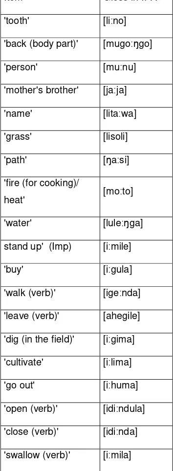
was elicited in seven locations have identical glosses in all seven word lists from those locations: [paːpa] ‘grandmother’ and [lugeːndo] ‘journey’. From the six locations where the long word list was taken, the following 19 items had identical glosses in all six speech varieties (see Table 7).
Item Gloss in IPA
Table 7 – Identical glosses in all six locations where the long word list was taken.
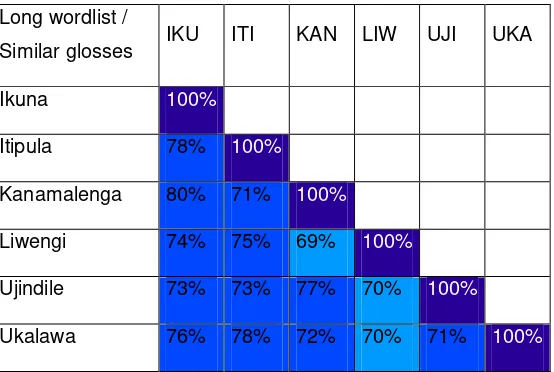
Long wordlist /
Table 8 – Percentages of identical glosses between the research locations of the long word list
Comparing the percentages of identical glosses of items between the research locations where the long word list was taken (Table 8), we find that Ikuna and Kanamalenga have the highest percentage of identical glosses (40%), the lowest percentages are between Liwengi and Ujindile (22%) and Liwengi and Kanamalenga (23%).
Long wordlist /
Table 9 – Percentages of similar glosses between the research locations of the long word list
Short wordlist /
Table 10 – Percentages of identical glosses between the research locations of the short word list
The comparison of the research locations where the short word list was taken in Table 10 shows that Ihanja and Wangama have the highest percentage of identical glosses between them (46%). Lwanzali has the lowest percentage of identical glosses both with Makanjaula and Utalingoro (12%).
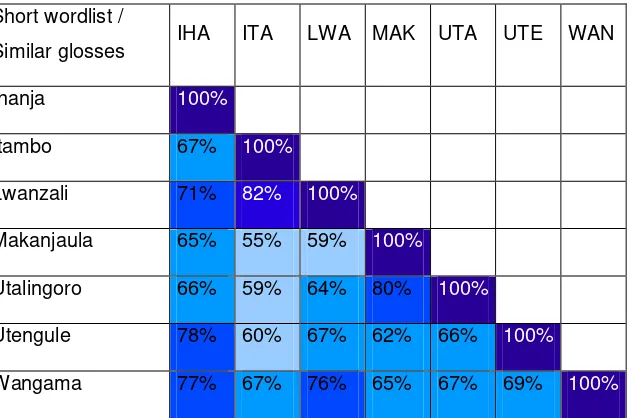
Table 11 – Percentages of similar glosses between the research locations of the short word list
In Table 11, comparing the similarity of glosses between locations where the short word list was taken, we see that the highest percentage of similar glosses is between the villages Itambo and Lwanzali (82%); the lowest percentage is between Itambo and Makanjaula (55%).
written in red, the locations where the short word list was taken are underlined. Similarly, percentages between two locations with long word lists are in red and percentages between two locations with short word lists are underlined. The other percentages are between locations where the long word list was elicited in one location and the short word list in the other location. Table 12 – Percentages of identical glosses between all the research locations
This combined matrix of identical glosses elicited in all the research location in Table 12 shows that the highest percentage of identical glosses is scored between Itambo and Itipula (59%), the lowest percentage between Lwanzali and Makanjaula and Lwanzali and
Similar
Table 13 – Percentages of similar glosses between all the research locations
When we look at Table 13 showing the percentages of similar glosses between all research locations, we find that Kanamalenga and Wangama have the highest percentage (90%) of similar glosses; Itambo and Makanjaula have the lowest percentage (55%). The varieties of Kanamalenga, Ukalawa and Itipula have rather high scores overall.
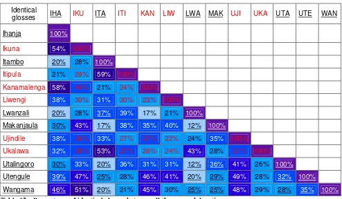
Identical
glosses IHA IKU ITA ITI KAN LIW LWA MAK UJI UKA UTA UTE WAN
Ihanja 100%
Ikuna 54% 100%
Itambo 23% 28% 100%
Itipula 21% 26% 59% 100%
Kanamalenga 58% 43% 21% 29% 100%
Liwengi 38% 38% 31% 33% 37% 100%
Lwanzali 18% 28% 52% 39% 17% 21% 100%
Makanjaula 37% 43% 30% 38% 35% 40% 18% 100%
Ujindile 38% 45% 33% 40% 47% 35% 24% 35% 100%
Ukalawa 32% 34% 53% 44% 27% 32% 43% 28% 32% 100%
Utalingoro 43% 33% 31% 36% 31% 31% 13% 44% 41% 26% 100%
Utengule 48% 47% 32% 28% 46% 41% 22% 38% 49% 28% 42% 100%
Wangama 47% 51% 28% 21% 45% 30% 30% 24% 48% 29% 35% 41% 100%
Table 14 - Percentages of identical glosses based on the 40 items asked in all research locations.
Similar
Table 15 - Percentages of similar glosses based on the 40 items asked in all research locations
In the matrix in Table 15 showing the percentages of similar glosses of the 40 items elicited in all thirteen research locations, we find that Kanamalenga and Wangama still have the highest percentage (90%) of similar glosses but this time Makanjaula and Utalingoro score just as high (90%). The lowest percentage here is shared between Ikuna and Itambo (56%), and Wangama shares high scores overall with all other locations.
Rather than presenting the results of the analysis and searching for patterns by putting them into tables and matrices, another way of doing this is to choose items from the word list that showed lexical variation in the glosses and show their geographical distribution in a linguistic map.
another language.34 The maps thus generated (Map 15 to Map 22) are below. On the maps,
the Swahili gloss which was used to elicit the Bena glosses is given, accompanied by its English equivalent. Each gloss has a certain colour for easier distinction.
Map 15 – The different glosses for ‘lake’ according to all locations.
Map 15 shows the seven different glosses given for the word ‘lake’ in ten of the Bena locations. Unfortunately, in Itipula, Ukalawa and Utalingoro this item was not elicited. Interestingly, the similar glosses in Ikuna, Ihanja and Ujindile lie more in the centre of the Bena area than the other locations. Note that the gloss [mukoga mukomi] given in Utengule can be translated as ‘big river’ and might be a paraphrase rather than the actual word used.
34
The ‚Leipzig-Jakarta list’ of basic vocabulary is one result of the Loanword Typology (LWT) project, a comparative study of lexical borrowability in the world's languages coordinated by the Max Planck Institute for Evolutionary Anthropology, Department of Linguistics (Uri Tadmor and Martin
Map 16 – The different glosses for ‘lion’ according to all locations.
In Map 16, the most widespread gloss for ‘lion’ is [ɲalupala] which can be found in five of the thirteen locations. In the three locations in the south (Liwengi, Makanjaula and
Map 17 – The different glosses for ‘eyebrow’ according to all locations.
Map 18 – The different glosses for ‘leaf’ according to all locations.
Four different glosses were given for ‘leaf’ which is the 64th item of the ‘Leipzig-Jakarta list’.
Map 18 shows the gloss [likwaːti] and its variants were given in the villages in the east of the Bena area: Ukalawa, Lwanzali and Itambo. Two of the glosses, [lituːndu] and [lihaːmba] with its variants are found in the northwestern part of the Bena area. In the central
Map 19 – The different glosses for ‘cat’ according to all locations.
As can be seen from Map 19, eight of the thirteen locations, from the east to the south and the most western location, gave the gloss [kimiːsi], [limisi] or their variants for ‘cat’. The other five locations gave two different glosses. In Kanamalenga in the north and in Ujindile in the west the gloss [ɲawu] was elicited, in Ihanja and Ikuna which lie more in the centre of the Bena area the gloss [himugogo] and the similar gloss [limkoko] were elicited. In Utengule, in the north but more central than Kanamalenga, the first response for the word ‘cat’ was [ɲawu], but then the participants gave the gloss [ʃimugogo] as their word for ‘cat’. As Utengule is close to Ihanja, Ikuna and Kanamalenga it lies in the sphere of influence of both glosses used in these locations, which explains the participants’ knowledge of both glosses.
Map 20 – The different glosses for ‘he/she knows’ according to primary locations.
This item, ‘he/she knows’, is the 58th item in the ‘Leipzig-Jakarta list’. Map 20 shows that
Map 21 – The different glosses for ‘he/she makes’ according to primary locations.
The item ‘he/she makes’ is the 25th item on the ‘Leipzig-Jakarta list’. In Map 21, the glosses
of Ikuna (central) and Liwengi (south) show hardly any variation. I also counted the glosses of Ukalawa (east) and Kanamalenga (north) as similar to each other. The gloss [iːtengeneza] which was elicited in Itipula (central-south) is clearly the Swahili prompt with Bena
morphology. Likewise, the gloss from Ujindile (west) is also a Swahili word which was
adjusted to the Bena language: kutenda in Swahili means ‘to do, to make’, kutengeneza
Map 22 – The different glosses for ‘ear’ according to primary locations.
For the gloss ‘ear’ in Map 22, which is the 22nd item in the ‘Leipzig-Jakarta list’, three
different glosses were elicited. In Ukalawa and Itipula (east and central east/south) we elicited [litwi] and its variant [liːtwi]. The participants in the word list collection of the other three locations, Kanamalenga (north), Ikuna (centre) and Ujindile (west), gave variations of one gloss which show the phonological differences between these locations ([ç]-[h] and [dʒ]-[ts], (see Map 10 and Map 12 respectively). [libulugutu] in Liwengi in the south is different from the rest.
4.3
Analysis using Gabmap
I used Gabmap as the second method for the analysis of the data from the Bena word lists. The use of a web application and the use of the Levenshtein distance for measuring
linguistic distances is a very different approach from the Blair Method.
To be able to display the data in maps, I created a map35 with the help of the GPS points
were uploaded to Gabmap. In uploading the data to Gabmap I used the default settings for string data: ‘tokenized string data’. ‘Tokenized string data’ means that vowels are aligned
and compared with vowels and consonants with consonants36. Any insertion, deletion or
substitution has the cost of 1, but if a vowel is substituted by a consonant the cost will be 2. Also, diacritics (e.g. [ː], vowel length) are treated as modifiers of the preceding vowel or consonant and if the only difference is in the diacritics then a cost of 0.5 will be assigned. The following figure (Figure 2) is an example of how Gabmap aligns the glosses and calculates the Levenshtein distance for each pair of glosses.
Figure 2 – Examples of tokenized alignment of glosses of the item ‘leaf’ using Levenshtein distance.
36
From the aggregated Levenshtein distances Gabmap calculated the following distance matrix (Table 16 below). I highlighted elements to show the highest and the lowest numbers between locations.
Table 16 – Distance matrix for all locations generated by Gabmap using Levenshtein distance.
According to this matrix, Ihanja and Kanamalenga, both located in the north of the Bena area, have the least linguistic distance. Not surprisingly we find the biggest linguistic distance between a location in the east, Lwanzali, and a location in the west, Utalingoro.
The linguistic differences can be seen better in the two difference maps Gabmap also produces: a network map (Map 23) and a beam map (Map 24). Network maps connect adjacent sites, using darker colours for linguistically more similar sites. In a beam map a line is drawn between each two sites where, again, the darker the line, the more
Map 23 – Network map of the Bena area (names of locations added).
From these maps one can see that there are two groups of linguistically closer locations within the Bena area, one in the east and one in the northwest.
Using weighted average37 as a clustering method for the linguistic distances, three main
clusters emerge. Map 25 shows these three clusters. The clustering itself is seen in the dendrogram in Figure 3. The colours of the clusters in the map correspond to those in the dendrogram.
Map 25 – Cluster map of the Bena area using weighted average (names of locations added).
Figure 3 – Dendrogram of the clusters using weighted average.
In the dendrogram we find again Ihanja and Kanamalenga as the linguistically closest locations, clustered together with Wangama, then with Ujindile and Utengule and Ikuna. We also see a major division between the locations in the east (Itambo, Ukalawa, Itipula and Lwanzali) and the rest of the locations. This is reflected in the map.
To validate clusters Gabmap also provides analysis with multidimensional scaling (MDS) which are plotted in two-dimensions. MDS plots are provided, both with the corresponding colours of the cluster maps and without colour. In Figure 4 we see them both. Numbers in the coloured MDS plot also correspond to the numbers for certain locations in the cluster map (Map 25).
Figure 4 – MDS plots, left with colours corresponding to the cluster map (Map 25) and cluster
dendrogram (Figure 3) and right without colours but locations labels.
According to this MDS plot there is a major division between the ‘blue’ locations of the east and south (Lwanzali, Itambo, Ukalawa, Itipula, Liwengi, Utalingoro and Makanjaula) and the ‘green’ locations in the north, central and west (Wangama, Kanamalenga, Ihanja, Utengule, Ujindile and Ikuna). We can also see a difference between the two ‘blue’ clusters, but here it is a little bit more difficult to draw the lines as these locations generally seem to be not all as linguistically close as the ‘green’ locations of the northern, central and western part of the Bena area.
differences in the clustering results.38 In the resulting probabilistic dendrogram (Figure 5),
the percentages show the relative certainty of certain clusters. The fuzzy cluster map (Map
26) visualises these clusters.39 The colours in the map correspond to the colours in the
dendrogram.
Figure 5 – Probabilistic dendrogram of the clusters (using the default settings).
Map 26 – Fuzzy cluster map of the Bena area (names of locations added).
38
In the dendrogram in Figure 5 we see that the cluster of the four eastern locations (Itambo, Itipula, Lwanzali and Ukalawa, in green) is stable, as is the major division between these four locations and the other locations. The cluster of the northern locations (Ihanja,