Competing and Defective Risks
John T. Addison
Pedro Portugal
a b s t r a c t
This paper examines the determinants of unemployment duration in a com-peting risks framework with two destination states: inactivity and employ-ment. The innovation is the recognition of defective risks. A polynomial hazard function is used to differentiate between two possible sources of in-finite durations. The first is produced by a random process of unlucky draws, the second by workers rejecting a destination state. The evidence favors the mover-stayer model over the search model. Refinement of the former approach, using a more flexible baseline hazard function, pro-duces a robust and more convincing explanation for positive and zero transition rates out of unemployment.
I. Introduction
This paper considers a model of unemployment duration in which exit from unemployment can result from finding a job or becoming inactive, two destinations that have been shown to be behaviorally distinct states (Flinn and Heck-man 1983). Use of a competing risks framework, while not yet commonplace in the duration literature, is becoming more familiar (see, for example, Han and Hausman 1990; Meyer 1990; Fallick 1991; Narendranathan and Stewart 1993). What is alto-gether less familiar is the notion exploited here that risks may be defective, in the
John T. Addison is Hugh C. Lane professor of economic theory, Moore School of Business, University of South Carolina, and a research fellow at the Institut zur Zukunft der Arbeit (IZA). Pedro Portugal is a senior economist with the Departamento de Estudos Econo´micos do Banco de Portugal, and is an as-sociate professor at the Universidade Nova de Lisboa. The authors thank the Fundac¸a˜o para a Cieˆncia Tecnologia for financial support. They are grateful for the helpful comments of Joa˜o Santos Silva and Manuel Arellano and those of two anonymous reviewers. Lucena Vieira provided excellent computa-tional assistance. The data used in this article can be obtained August 2003 through July 2006 from Pedro Portugal, Banco de Portugal, Av. Almirante Reis 71, 1150 Lisboa, Portugal.
[Submitted February 2000; accepted November 2001]
ISSN 022-166X2003 by the Board of Regents of the University of Wisconsin System
Addison and Portugal 157
sense that certain destination states may not be considered by unemployed individu-als, whose observed and unobserved characteristics may anyway rule them out as candidates for employment. The notion that unemployed individuals may be perma-nently trapped in joblessness is explored theoretically in Blanchard and Diamond (1994), Ljungqvist and Sargent (1998), and Ridder and van den Berg (2001).
We would argue that the idea that risks are defective is likely to be especially relevant to high unemployment/long jobless duration European labor markets in gen-eral and to their more sclerotic component markets such as Portugal—the subject of this empirical inquiry—in particular where unemployment may come to represent a near pathological end state.1(In other nations, where unemployment may be less entrenched, the notion of defective risks might still usefully be deployed to analyze transitions into certain types of employment, such as open-ended employment versus fixed-term contracts or full-time versus part-time work.) If certain destination states are not viable, the standard problems associated with aggregating over a number of exit modes will only be compounded. Specifically, as we shall show, there will be a bias in favor of negative duration dependence and one will tend to underpredict the probability of not changing state.
In this paper, we will consider two distinct statistical duration models that lend themselves to infinite durations, and thus to a defective risk. Our favored model is a so-called ‘‘split-population model’’ in which some individuals do not contemplate (or are excluded from) certain labor markets options and thereby come to constitute different populations from those that do. In this case, the probability of moving from one state to another is zero from the outset. In particular, we will allow the proportion of stayers to be influenced by observed heterogeneity. This type of model, which generalizes the more conventional mover-stayer model allowing for regressors to influence the probability of being a stayer, was first applied by Schmidt and Witte (1989) to the recidivism phenomenon in criminal behavior. To our knowledge the only labor applications are by Yamaguchi (1992), Pudney and Thomas (1995), and Melkersson (1999), each of which has a narrower focus than the present paper.2 Yamaguchi considers the implications of permanent employment in Japan for labor market transitions. Pudney and Thomas investigate movements from unemployment to specific industry sectors. Melkersson studies the return to employment of a sample of Swedish disabled workers, distinguishing between three competing exits from unemployment: regular employment, sheltered employment, and inactivity.
But before considering the basics of our split-population model, however, it is important to point out that the presence of defective risks is quite compatible with other statistical duration models. In the second type of model considered here, we simply recognize that some specifications of the latent hazard (see Section III) can deliver defective latent distributions—see, for example, Flinn and Heckman’s (1982) use of a polynomial hazard function in a competing risks framework.
Estimation of this type of model does not present major difficulties. In other words,
1. For an alternative statistical duration model that distinguishes between short- and long-term unemploy-ment, see Portugal and Addison (1995).
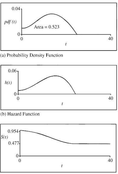
Figure 1
Illustration of a Nonproper Distribution
there is nothing anomalous about defective distributions and they may emerge natu-rally in optimizing models (Heckman and Singer 1985). As a case in point, Jovanovic (1979) derives an infinite horizon worker-firm matching model with a defective (in-verse-Gaussian) job tenure distribution.
Addison and Portugal 159
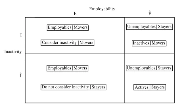
Figure 2
Split-Population Typology
relevance of this possibility is clearly an empirical issue. We will tentatively label this model a ‘‘Nonproper distribution model.’’
Nonproper (or defective) distributions are not the sole source of infinite durations because other approaches admit defective risks. For example, consider the determi-nants of the age at which women give birth to their first child. The problem is that one may be sampling from two distinct subpopulations, one of which is made up of infertile couples who will have infinite durations. This very scenario is analyzed formally by Heckman and Walker (1990). The generalization of this mover-stayer model to more than one exit state is fairly simple. We argue that some unemployed individuals will consciously rule out the option of labor market withdrawal. At the same time, there will also be unemployed workers who, by virtue of their past choices or current skill endowments, will be unable to secure employment. Such individuals can be termedunemployables.
The basic elements of our split-population model are presented informally in the 2⫻2 matrix of Figure 2. The horizontal axis denotes the population of employables and unemployables, denoted byEandEˆ, respectively. Employables are those indi-viduals who may transition from unemployment (U) to employment (E), and whom we therefore termU-E movers. Unemployables are those persons who will never transition from unemployment to employment, and are referred to asU-E stayers. On the vertical axis is given the population of those who either consider or rule out the option of labor market withdrawal, respectivelyIandIˆ. They will be termed
U-I movers andU-I stayers. (By analogy with the biostatistical literature, EandI
may also be termed employment and inactivitysusceptibles, while Eˆ andIˆcan be said to represent the population of employment and inactivityimmunes.)
never enter inactivity; in this sense they are respectivelyU-E moversandU-I stayers. The U-E hazard function to be estimated is correctly estimated across these two cells or populations. As for the third, top-right cell this comprisesU-E stayers(or employment immunes), andU-I movers (or inactivity susceptibles), who will ulti-mately move into that destination state. The inactivity hazard function is properly estimated over the first and third cells. Finally, the fourth cell is made up of the long-term unemployed, or more accurately the permanently unemployedwho are
U-E andU-I stayers(or employment immunes and inactivity immunes). In other
words, for individuals to stay in the unemployment state forever requires that they are defective in two respects, both in terms of the transition from unemployment into employment and also the unemployment to inactivity transition. Clearly, if the latent hazards are independent, the probability of never leaving the unemployment spell is just the product of the probability of being aU-E stayerwith the probability of being aU-I stayer.
In this paper, we seek to test for the presence of defective risks such as might result from a random process of unlucky draws and defective risks produced by two very different populations. To effect this comparison, we will first deploy a simple fourth order polynomial baseline hazard function. The basis of the test of the unlucky draws scenario is based simply on the distribution parameters. The basis of the test of the split-population model is a specification that uses the same polynomial baseline hazard but which allows the regressors to affect the population of stayers and not simply the escape rates from unemployment of employment and inactivity movers. In both cases, a correction for unobserved individual heterogeneity is provided. The split-population model is then further refined to allow a more flexible baseline hazard function in the form of a (13-segment) piecewise constant hazard. Finally, since we have no guidance as to proportionality or otherwise, we also estimate a discrete change specification for the impact of the regressors.
The plan of the paper is as follows. Section II introduces the Portuguese data set and offers a modicum of detail on that country’s labor market. Section III offers a formal presentation of the methodology. Detailed presentation of our findings is pro-vided in Section IV. A summary drawing together the threads of the preceding argu-ments concludes.
II. Data
Our data are taken from the nationally representative Portuguese quarterly employment surveys (Inque´rito ao Emprego), conducted by the National Institute of Statistics (INE) (Instituto Nacional de Estatistica). The sample period is 1992(2)–97(4), the starting date being dictated by changes in survey design after the first quarter of 1992.
distin-Addison and Portugal 161
guish between the two destination states of employment and inactivity.3We note in passing that the employment survey is similar to other labor force surveys in provid-ing a snapshot of the stock of unemployed at two moments in time, in this case separated by a quarter. Familiarly, remaining duration of unemployment of those who do not transition out of unemployment has to be inferred. Registered elapsed unemployment duration is top-coded for individuals with 98 months of unemploy-ment or more, though this is a very small proportion of the sample (amounting to less than one percent).
Each survey provides information on the length of the current unemployment spell in months and the unemployment benefit status of the worker. It is also possible to track time to exhaustion of benefits. Although we do not exploit the latter information here, instead using access to unemployment benefits (both unemployment insurance proper and means-tested unemployment assistance), note that the seven-element structure of our age regressor is designed exactly to mimic the stepped increases in benefit entitlement with age. For all intents and purposes, the replacement rate is fixed in Portugal (at 65 percent). Neither it nor the duration of unemployment insur-ance benefits, which is exclusively age determined, changed over the sample period.4 In addition to access to benefits and age, the employment survey contains informa-tion on a number of other variables that may be expected also to shift the baseline hazard up or down. Those selected in the present paper are level of schooling, marital status, tenure on the job, whether the individual is a new entrant, and the reason for job loss leading to the unemployment event. The local unemployment rate, derived from a source other than the employment survey, was also allowed to shift the base-line hazard function(s).
Because we wish to account for defective risks, each of the above arguments specific to the individual (namely, age, receipt of benefits, schooling, tenure on the last job, and marital status) plus the unemployment rate were used to estimate the split-population regression equations. The general point is that we are interested in considering the factors that affect the probability of being a long-term survivor. Age is expected to be critical in this regard, and is now expressed in continuous form rather than as a grouped variable. Unemployment benefits and the local unemploy-ment rate are also of special interest: The former because it is the key policy variable, and the latter because it is expected to inform on discouragement.
The sole restrictions placed on the data were that the individual be a male unem-ployed at the time of the quarterly survey, aged between 16 and 64 years, and a resident in mainland Portugal. Given the possibility of sample attrition, we also en-sured that individuals appearing in contiguous surveys with the same identifier were in fact the same individual. The sample size is 9,451 individuals. Descriptive statis-tics are provided in Appendix Table A1.
3. For an analysis of job search methods used by unemployed workers that exploits the wider array of destination states contained in the survey, see Addison and Portugal (2002).
Over the course of the sample period, the Portuguese unemployment rate rose by almost two-thirds (from 4.1 percent in 1992 to 6.7 percent in 1997). The mean (elapsed) duration of unemployment increased continuously (from 12.2 months to 16.5 months) and, not surprisingly, the distribution of unemployment changed fairly profoundly. In particular, the share of long-term unemployment (12 months or more) rose by almost 74 percent (from 24.9 to 43.3 percent). Note that the proportion of workers covered by the unemployment benefit system has changed little since 1993, and also that the maximum duration of benefits and the replacement rate rules were unchanged over the entire sample period.
Since 1997 the unemployment rate has improved materially and currently approxi-mates the U.S. value. Nevertheless, the scale of the long-term unemployment prob-lem persists. Moreover, Portugal continues to be regarded as the exemplar of a sclerotic labor market, with the highest level of employment protection in OECD countries (see OECD 1999). Furthermore, it has continued to be dogged by what has been termed a ‘‘stagnant pool’’ of unemployment (Blanchard and Portugal 2001, p. 187), with low flows in and out and (the corollary) long unemployment duration (see also Bover, Garcı´a-Perea, and Portugal 2000). This, then, is the backdrop to the present empirical inquiry.
III. Methodology
A. Two Simple Hazard Models
A critical concept in statistical analysis of a duration phenomenon is the hazard
function.In the study of unemployment duration, the hazard function gives the
in-stantaneous probability of exiting unemployment att, given that the individual stayed unemployed untilt
(1) h(t)⫽lim
∆t→0
P(tⱕT⬍t⫹∆t|Tⱖt)
∆t ⫽
f(t) 1⫺F(t)⫽
f(t)
S(t),
wheref(t) is the probability density function, F(t) is the distribution function, and
S(t) is the survival function. A useful function is the integrated hazard function
(2) Λ(t)⫽
冮
t0
h(u)du,
which relates to the survivor function simply by
(3) S(t)⫽e⫺Λ(t).
In this paper we consider two flexible forms for the hazard function. The first is a fourth order polynomial hazard function
(4) h(t)⫽α0⫹α1t⫹α2t2⫹α3t3⫹α4t4. α0ⱖ0
Addison and Portugal 163
(5) h(t)⫽
eλ1 if 0ⱕt⬍c
1
eλ2 if c
1ⱕt⬍c2
eλ3 if c
2ⱕt⬍c3 , .
.
eλm⫺1 if c
K⫺1ⱕt
where the time axis is divided into Kintervals by pointsc1,c2. . . ,cK⫺1.5For the piecewise-constant model, a nonproper distribution is precluded since the hazard rate is positive for the last (open-ended) interval.
B. A Two-destination Model
In this paper we shall also distinguish between two exit modes out of unemployment: employment and inactivity. Thus, we define cause-specific hazard functions to desti-nationj
(6) hj(t)⫽ lim ∆t→0
P(tⱕT⬍t⫹∆t|Tⱖt,J⫽j)
∆t , j⫽1, 2
which yield the aggregate hazard function
(7) h(t)⫽
冱
2j⫽1
hj(t).
and the survivor function
(8) S(t)⫽
兿
2j⫽1
Sj(t), whereSj(t) ⫽e⫺Λ
j(t), andΛj(t)⫽冮0thj(u)du.
The model has a conventional competing risks interpretation. In this framework, a latent duration (Tj) unemployment attaches to each exit mode. We only observe the minimum of each latent variable. If risks are assumed to be independent, with continuous duration, this model simplifies to two separate single-cause hazard mod-els (but see below).6
5. As noted earlier, we use month as the time calendar unit. In specifying the baseline hazard function, we used three initial one-month intervals, seven subsequent intervals of three months’ duration, then two intervals of six months, and a final, open-ended interval. In other words, the knot points are 1, 2, 3, 6, 9, 12, 15, 18, 21, 24, 30, and 36.
C. Proportional Hazards Specification
A common way to accommodate the presence of observed individuals is to specify a proportional hazards model
(9) hj(t;x)⫽h0j(t)ex′βj,
whereh0j(t) denotes the baseline specific hazard function, that is, the hazard function corresponding to null values for the covariatesx. In this case, the covariates affect the hazard function proportionally (that is,dh(x)/dxk⫽βkh(x)). An implication of this assumption is that the impact of the covariates does not change (in relative terms) with the progression of the spell of unemployment. We shall return to the discussion and test of this restriction below.
D. Discrete Duration Model
Our information on elapsed duration of unemployment is grouped into monthly inter-vals (while transitions can solely be identified over a fixed interval of three months). LetM⫽mdenote the occurrence of an exit in a given month [ct⫺1,ct), wheremis the realization of a discrete random unemployment duration variableM∈(1, . . . ,
K). The probability that an event occurs in the mthinterval (that is, an exit occurs over the course of the three-month window), and that such an exit is to destination
r, will be given (neglecting, for the sake of parsimony, thetandxindexes) by
(10) fr m⫽
Sr m⫺3⫺Srm
Sr m⫺3
Sm⫺3⫽hrmSm⫺3.
The functionsfr
mand (1⫺Srm) provide a convenient characterization of the proba-bility density and the cumulative functions associated with the marginal distribution for each latent duration,Tj, in terms of the specific hazard functionhrm. A censored observation (namely, a spell of unemployment that is still in progress after the three-month window) occurs with probabilitySm⫽∏2j⫽1Sjm, which is simply the product of the two specific survivor functions.
E. Observation Over a Fixed Interval
Addison and Portugal 165
(11) L(θ |t,j,x)⫽
冦
兿
K⫺1m⫽1
兿
2j⫽1
冤
Sj
m⫺3⫺Sjm
Sj m⫺3
冥
δmj
冧冦
兿
m⫽2K冤
Sm
Sm⫺3
冥冧
1⫺δm,
whereθ is a vector of parameters that include regression coefficients and baseline hazard parameters, andδmjis an indicator that assumes the value of one if the individ-ual exits to destination jduring themthinterval, and zero otherwise. The indicator
δm⫽∑2j⫽1δmjidentifies completed durations, so that 1⫺δmequals 1 for a censored observation. Notice that, after conditioning on having survived untilm⫺t, theSm⫺3 term cancels out for completed durations. The contribution to the likelihood function from a censored observation is simply the product, conditional on surviving up to
m ⫺3, of the two specific survival terms (∏2
j⫽1Sjm), that is, the probability of not exiting to either employment or inactivity.
E. Unobserved Individual Heterogeneity
We also attempt to accommodate the presence of unobserved individual heterogene-ity by assuming, as conventional, a multiplicative error term associated with each specific hazard function
(12) hj(t;x)⫽h0j(t)ex′βjvj.
We further assume that the errorsvjare gamma distributed with mean 1 and variance
σ2
j and are uncorrelated.7
We proceed by redefining the specific survivor function using the well-known result for gamma mixturesS¯j
m⫽(1⫹σ2jΛjm)⫺1/σ
2
j (see Lancaster 1990, p. 66). After this transformation, the likelihood function is derived as for Equation 11 above
(13) L(θ,σ2|t,j,x) ⫽
冦
兿
K⫺1
m⫽1
兿
2j⫽1
冤
(1⫹σ2jΛjm⫺3)⫺1/σ
2
j ⫺(1⫹σ2 jΛjm)⫺1/σ
2
j
(1⫹σ2jΛjm⫺3)⫺1/σ
2
j
冥
δmj
冧
冦
兿
m⫽2K兿
2
j⫽1
冤
(1⫹σ2jΛjm)⫺1/σ
2
j
(1⫹σ2
jΛjm⫺3)⫺1/σ
2
j
冥冧
1⫺δm.
F. Split-Population Model
Up to this point we have assumed that all destination states are viable ex ante. In other words, even though we allow for the possibility of infinite duration via a nonproper distribution (for given parameters of the polynomial hazard function), until now we neglected the existence of stayers. That is, we have assumed that with respect to transitions to both employment and inactivity all individuals were (potential)movers. We now have to account for the possibility that certain or all choices may be ruled
out. This approach has been used in the econometric literature in the context of a ‘‘split-population’’ framework for a single risk (Schmidt and Witte 1989).8
In the context of a grouped duration model, a straightforward way to incorpo-rate the possibility of defective risks is to redefine the specific survival function as
S˜j
m⫽1⫺Pj⫹PjSjm, wherePjis the proportion of movers associated with destina-tionj. Thus, the survival probability is given by the proportion ofjstayers, (1⫺Pj), who do not exit into destinationjwith probability l, plus the proportion of movers,
Pj, multiplied by the corresponding probability of transition intojatm,Sjm. TakingPj as additional unknown parameters to be estimated, the new parame-terization of the specific survivor function can be employed in a likelihood function identical to Equation 11. In order to guarantee that Pjlies between zero and one, we employ the logit reparameterization forPj⫽exp(µj)/l⫹exp(µj). This use of a logit link function is inconsequential in terms of finding evidence of stayers since it does not preclude the possibility ofPjbeing as close to one (or zero) as needed. A natural extension of this model is to allowPjto depend on a set of regressors
z, leading to an extended logit link functionPj⫽exp(µj⫹z′γj)/1⫹exp(µj⫹z′γj) (see Yamaguchi 1992). That is, we can again use the structure of Equation 11 to specify the likelihood function
(14) L(θ |t,j,x)⫽
冦
兿
K⫺1m⫽1
兿
2j⫽1
冤
Pj(Sjm⫺3⫺Sjm) 1⫺Pj⫹PjSjm⫺3
冥
δmj
冧
冦
兿
m⫽2K兿
2
j⫽1
冤
1⫺Pj⫹PjSjm 1⫺Pj⫹PjSjm⫺3
冥冧
1⫺δmi ,
whereθnow represents the vectorsβj,µj,γj, and the baseline hazard parameters. A censored observation results from the interplay of being a U-E stayer (namely, 1 ⫺P1), being anU-I stayer(1-P2), being anU-E moverand not exiting to E(P1
S1
m), and being anU-I moverand not exiting to I (P2S2m). The probability of observing an incomplete duration will be given by the product of the probabilities of not exiting to employment (being an U-E stayer plus being a survivor U-E mover) and not exiting to inactivity (being anU-I stayerplus being a survivorU-I mover).
G. Split Population and Unobserved Individual Heterogeneity
In order to account for both defective risks and gamma heterogeneity, we employ the transformationSˆj
m⫽1⫺Pj⫹Pj(1⫹σ2jΛjm)⫺1/σ
2
j. In short, inserting this defini-tion into Equadefini-tion 11 we define the following likelihood funcdefini-tion
(15) L(θ,σ2|t,j,x) ⫽
冦
兿
K⫺1
m⫽1
兿
2j⫽1
冤
Pj(1⫹σ2jΛjm⫺3)⫺1/σ
2
j ⫺(1⫹σ2jΛjm)⫺1/σ2j) (1⫺Pj⫹Pj(1⫹σ2jΛjm⫺3)⫺1/σ
2
j)
冥
δmj冧
Addison and Portugal 167
冦
兿
K⫺1m⫽1兿
2j⫽1
冤
(1⫺Pj⫹Pj(1⫹σ2jΛjm)⫺1/σ
2
j)
(1⫺Pj⫹Pj(1⫹σ2jΛjm⫺3)⫺1/σ
2
j)
冥冧
1⫺δm.
In this case, there are two sources of unobserved heterogeneity competing with each other to account for unforeseen factors. On one hand, there is a distinction between movers and stayers, in terms of both employment and inactivity. On the other hand, conditional on being a mover, there is an error term in the specific hazard function that accounts for omitted variables.
Finally, we note that the ML routine from the econometric package TSP (Time Series Processor) was employed to obtain the maximum likelihood estimates. In each case, starting values from a simple single risk specification were used.
H. Identifiability Issues
The specification of our models is based on a delicate compromise between parsimony and computational simplicity on the one hand, and flexibility and goodness of fit on the other. In the interests of tractability, we have assumed (a) independent competing risks, (b) (conditional) proportional hazards, and (c) para-metric (gamma) unobserved individual heterogeneity. We will not elaborate on these assumptions other than to note that they are fairly conventional and well studied (see, in particular, Heckman and Honore´ 1989 and Crowder 2001, on the identifiability of competing risk models).
A crucial issue for the present study is the identifiability of defective risks. There are two questions that we have to address. First, is it possible to identify nonparamet-rically the presence of defective risks? And second, subject to an affirmative answer to this question, can one be confident that the follow-up period is long enough to enable the detection of long-term survivors? Under ideal data conditions (say, obser-vation over an infinite time horizon) the answer to the first question is obviously yes, because one can then distinguish between finite and infinite durations. But even under less than ideal conditions one can still detect nonparametrically the presence of long-term survivors if the follow-up period is sufficiently long.
Through functional form assumptions one can obtain parametric identifiability of defectiveness at the cost of some additional arbitrariness. Here we have explored two routes: the mover-stayerparadigm and theunlucky drawsapproach. Whereas the latter approach lends itself to a number of structural job search interpretations under which the hazard rate converges to zero at too fast a rate to allow all individuals to transition, the former arrives naturally from a sequential decision framework or from a finite mixture model (McLachlan and Peel 2000). These are, in essence, two distinct ways to interpret duration data (with defective risks).
Nevertheless, it has to be admitted at the outset that one cannot tell which model applies solely from the duration data. In this sense, the two approaches are observa-tionally equivalent. Identification hinges on the functional forms of the hazard func-tions employed.9A crucial issue with defective risks models is the behavior of the model in the right tail of the duration distribution. The reason why we selected two flexible (sub)hazard functions—piecewise-constant and polynomial—was the need to avoid imposing too much structure on the data, notably at the right tail of the survival distribution. We hope that by proceeding in this way there is a lesser risk of artificially generating evidence of defective risks.
Finally, we decided to impose the proportional hazards functional form on the conditional specific hazard function. This form of hazard is more natural and has greater appeal than results from imposing proportionality on the unconditional hazard function (Ibrahim, Chen, and Sinha 2001). It also provides a simple interpretation of the hazard regression coefficients. Proportionality is not necessarily indicated by theory and can and should be tested, as here.
IV. Findings
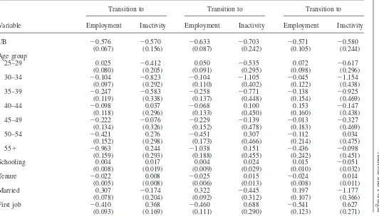
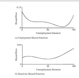
Results of fitting the basic competing risks model, assuming a fourth order polynomial hazard function, are provided in the first two columns of Table 1. The first point to note is that there is no evidence that the duration marginal distribu-tions are defective. Thus, for transidistribu-tions into employment, the coefficient estimate of the quartic term is (statistically) greater than zero, so that the integrated hazard converges to infinity astgoes to infinity. For transitions into inactivity, the quartic coefficient estimate although negative is not statistically different from zero. Indeed, for this destination state the linear, quadratic, and cubic terms are uniformly insig-nificantly different from zero, with only the constant term being statistically signifi-cant at conventional levels. The baseline hazard functions for employment and inac-tivity are presented in panels (a) and (b) of Figure 3. Both functions are well behaved. The employment hazard is decreasing over a large portion of the relevant range (the data are top-coded at 98 months). For its part, the inactivity hazard never approaches
Addison
and
Portugal
169
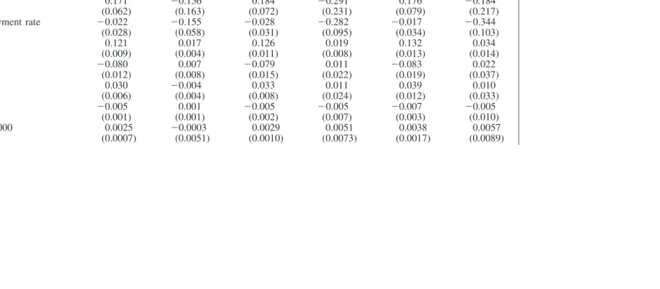
Table 1
Two-Destination Polynomial Hazard Regression Models (n⫽9,451)
Transition to Transition to Transition to
Variable Employment Inactivity Employment Inactivity Employment Inactivity
UB ⫺0.576 ⫺0.570 ⫺0.633 ⫺0.703 ⫺0.571 ⫺0.580
(0.067) (0.156) (0.087) (0.242) (0.105) (0.244)
Age group
25–29 0.025 ⫺0.412 0.050 ⫺0.535 0.072 ⫺0.617
(0.080) (0.205) (0.091) (0.295) (0.098) (0.296)
30–34 ⫺0.104 ⫺0.823 ⫺0.104 ⫺1.105 ⫺0.045 ⫺1.154
(0.097) (0.292) (0.110) (0.402) (0.122) (0.438)
35–39 ⫺0.247 ⫺0.583 ⫺0.258 ⫺0.771 ⫺0.138 ⫺0.925
(0.119) (0.338) (0.137) (0.448) (0.154) (0.469)
40–44 ⫺0.098 0.037 ⫺0.068 0.100 0.153 ⫺0.147
(0.118) (0.296) (0.133) (0.450) (0.160) (0.438)
45–49 ⫺0.222 ⫺0.076 ⫺0.229 ⫺0.139 ⫺0.013 ⫺0.327
(0.134) (0.326) (0.152) (0.478) (0.183) (0.469)
50–54 ⫺0.421 0.276 ⫺0.451 0.307 ⫺0.112 0.034
(0.152) (0.298) (0.173) (0.466) (0.214) (0.475)
55⫹ ⫺0.963 0.244 ⫺1.038 0.151 ⫺0.436 ⫺0.098
(0.159) (0.293) (0.188) (0.455) (0.242) (0.451)
Schooling 0.004 0.017 0.004 0.024 0.015 ⫺0.051
(0.008) (0.019) (0.009) (0.029) (0.010) (0.032)
Tenure ⫺0.022 0.008 ⫺0.025 0.015 ⫺0.024 0.014
(0.005) (0.008) (0.006) (0.013) (0.008) (0.011)
Married 0.307 ⫺0.174 0.322 ⫺0.445 0.197 ⫺1.177
(0.078) (0.204) (0.092) (0.312) (0.107) (0.366)
First job ⫺0.410 0.368 ⫺0.460 0.688 ⫺0.541 0.627
The
Journal
of
Human
Resources
Table 1(continued)
Transition to Transition to Transition to
Variable Employment Inactivity Employment Inactivity Employment Inactivity
Layoff 0.008 ⫺0.664 ⫺0.013 ⫺0.867 ⫺0.071 ⫺0.775
(0.090) (0.233) (0.102) (0.328) (0.114) (0.287)
End fixed 0.171 ⫺0.156 0.184 ⫺0.291 0.176 ⫺0.184
(0.062) (0.163) (0.072) (0.231) (0.079) (0.217)
Unemployment rate ⫺0.022 ⫺0.155 ⫺0.028 ⫺0.282 ⫺0.017 ⫺0.344
(0.028) (0.058) (0.031) (0.095) (0.034) (0.103)
Constant 0.121 0.017 0.126 0.019 0.132 0.034
(0.009) (0.004) (0.011) (0.008) (0.013) (0.014)
t/10 ⫺0.080 0.007 ⫺0.079 0.011 ⫺0.083 0.022
(0.012) (0.008) (0.015) (0.022) (0.019) (0.037)
t2/100 0.030
⫺0.004 0.033 0.011 0.039 0.010
(0.006) (0.004) (0.008) (0.024) (0.012) (0.033)
t3/1000
⫺0.005 0.001 ⫺0.005 ⫺0.005 ⫺0.007 ⫺0.005
(0.001) (0.001) (0.002) (0.007) (0.003) (0.010)
t4/100,000 0.0025
⫺0.0003 0.0029 0.0051 0.0038 0.0057
Addison
and
Portugal
171
Sigma 0.389 1.569 0.465 0.974
(0.154) (0.339) (0.164) (0.385)
Split-population equation
Mu 4.301 0.653
(0.972) (0.466)
UB ⫺1.424 ⫺0.298
(0.504) (0.666)
Age ⫺0.187 0.029
(0.047) (0.030)
Schooling ⫺0.132 0.226
(0.057) (0.081)
Tenure ⫺0.022 ⫺0.028
(0.024) (0.042)
Married 1.890 4.900
(0.663) (7.073)
Unemployment rate ⫺0.575 0.170
(0.446) (0.184)
Log-likelihood ⫺5,048.12 ⫺5,041.73 ⫺5,019.93
Figure 3
Polynomial Hazard Function
Note: Baseline hazard functions obtained from Table 1, Columns 1 and 2, respectively.
zero over the relevant range. Furthermore, one would not reject the null hypothesis of
αconstant (exponential) hazard function for this destination state (chi-square (4)⫽ 3.58; p⫽0.466).
Addison and Portugal 173
entering unemployment by reason of a mass layoff subsequently return to employ-ment at higher rates than do individual separations.
Results of implementing the parametric correction for unobserved individual het-erogeneity are shown in the third and fourth columns of Table 1. Note that although the sigma coefficient estimates are well determined, the correction does not yield any substantive changes on the earlier results. But there is clear suggestion of higher (error) variance in the case of employment transitions and, more generally, the re-gression coefficient estimates increase in absolute magnitude as well as in their im-precision. The coefficient estimates for the polynomial hazard functions again fail to indicate that the marginal duration distribution is defective for either the employ-ment or the inactivity transitions.
We take this evidence as suggesting that, within this type of specification, latent infinite durations are not present in the data. In other words, an individual does not face a nonzero probability of drawing an infinite duration. At this point, we therefore end our discussion of nonproper distributions and in what follows focus our attention on the split-population (or mover-stayer) alternative characterization. This, of course, does not preclude the use of a polynomial hazard function. It just happens that the estimation results appear to suggest that defective risks are present via the heteroge-neity of the underlying sub-populations in our sample. The nature of this heterogene-ity is simply the distinction between the sub-population of individuals who would always ultimately transition to a given destination state, and those would never make that transition.
The split-population model is presented in the last two columns of Table 1, again assuming a polynomial specification for the distribution function and correcting parametrically for unobserved individual heterogeneity. There is strong evidence of defective risks. Beginning with employment transitions, three variables—age, access to unemployment benefits, and schooling—increase the probability of being
a U-E stayer(or employment-immune), while marital status significantly reduces
that probability. With the exception of the perverse schooling effect, these results seem sensible. We shall have occasion to revisit the schooling result below.
⫺15(.187))/(1⫹(4.301⫺1.424⫺15(.187)), thus yielding the immune proportion of 48.2 percent.)
It appears that the main effect of age on transitions from unemployment into em-ployment works through the increase in the proportion ofU-E stayers(or employ-ment immunes) rather than through a reduction in the hazard rate of the employemploy-ment mover population. As can be seen in the penultimate column of Table 1, the coeffi-cient estimates for all but the highest age category are now statistically insignificant. Nevertheless, the receipt of unemployment benefits variable retains its explanatory power after accounting for the presence of employment immunes or stayers. This suggests that there are two mechanisms at work. On one hand, receipt of unemploy-ment benefits increases quite sizably the number of individuals who will never gener-ate an acceptable job offer (that is, increases the number ofU-E stayers). On the other hand, one also obtains the more conventional result that access to unemploy-ment benefits decreases transitions into employunemploy-ment; that is, it reduces hazard rates amongU-E movers.
Turning finally to transitions from unemployment to inactivity (U-I), shown in the final column of Table 1, it is clear that we are indeed largely sampling from a population that will never transition into inactivity, comprisingU-I stayersor inactiv-ity immunes. This is indicated by the low value of the constant term, which implies that no less than 48.2 percent of the unemployed population will never consider inactivity. Of the variables expected to influence the proportion of inactive immunes, only schooling is statistically significant and it operates to prevent flows from unem-ployment into inactivity. There is evidently a larger portion of individuals among more highly educated groups that never consider the inactivity option.
If one were to sample 35 year olds possessing (other) average characteristics for the continuous variables and who are assigned reference values for the binary vari-ables, some 34.2 percent of this group would beU-I stayers(or inactivity immunes). This proportion is decreasing in age: it is about 44.6 percent for workers aged 20 years, and falls to 25.2 percent for workers aged 50 years.
In general, the coefficients contained in the final column of Table 1 are estimated with less precision than before. In part, this result reflects the combination of a com-paratively small number of unemployed individuals entering inactivity (n⫽305, or 3.2 percent) with a heavily parameterized specification.
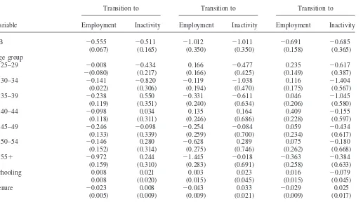
In Table 2 we report parallel results from fitting a 13-segment piecewise-constant baseline hazard function (rather than a fourth order polynomial) to the duration data. Thus, the first two columns of the table give results for the basic competing risk specification; the next two columns supplement this specification with a control for gamma unobserved individual heterogeneity; and the last two columns present the full defective risks specification in which the probability of observing infinite dura-tions (or individuals with zero transition rates—that is, stayers) is allowed to be influenced by six regressors.
Addison and Portugal 175
integrated hazard function converges to infinity astgoes to infinity. In other words, unlike the polynomial specification, by construction the piecewise-exponential func-tion does not allow individuals to draw infinite durafunc-tions (the density probability function has no mass point at infinite duration). Long-term (infinite) survivors are possible solely through the presence of stayers.
The regression coefficient estimates for the basic model in the first two columns are remarkably close to the corresponding estimates from the polynomial specifica-tion in Table 1, although the positive effect of mass layoffs on the employment hazard is now statistically significant. But some differences emerge with the correc-tion for unobserved individual heterogeneity in the next two columns. Not only are estimates of the error terms higher compared with the polynomial specification for both the employment and inactivity equations, but the regression coefficient esti-mates change markedly and are mostly higher in absolute terms. To take just one example, access to benefits is now associated with a downward deflection of both hazards of around 64 percent (as compared with 50 percent or less).
Turning to the last two columns of Table 2, however, we find that the regression coefficient estimates for the hazard function(s) are now much closer to the polyno-mial. The major differences between the two concern the regression coefficients for the split-population equation. In particular, the age and schooling coefficient esti-mates for employment are now smaller than before in absolute magnitude. Both outcomes seem sensible. As far as the schooling variable is concerned, this is no longer statistically significant; that is, we no longer obtain the troublesome result that those with higher levels of schooling are more likely to beU-E stayers. As far as age is concerned, we would surmise that the use of a more flexible baseline hazard goes some way toward correcting the inverse association between age and schooling level that appears to exaggerate the effect of age on the proportion ofU-E stayers
in the polynomial specification. In any event, the estimated population of unemploy-ables is much higher than before: 23.1 percent (9.1 percent) for 35 year-old unem-ployment benefit recipients (nonrecipients), and 51.8 percent (27 percent) for 50 year-old recipients (nonrecipients).
The split-population results for inactivity resemble those obtained for the corre-sponding polynomial specification in Table 1. Specifically, the estimated proportions
of U-I stayers are now: 37 percent (28.7 percent) for 35 year-old unemployment
benefit recipients (nonrecipients) and 26.7 percent (19.9 percent) for 50 year-old recipients (nonrecipients).
The estimated error variances are still much higher for the piecewise-constant specification vis-a`-vis the polynomial counterpart. It appears that the gamma vari-ance estimate is particularly sensitive to the manner in which the upper tail of the distribution of unemployment duration is modeled. Overall, since the results for the piecewise constant variant of the split-population model seem to be more convincing than for the polynomial, we shall use the former estimates to further address the critical role of age and unemployment benefits in affecting hazard rates and defective risks and to illustrate the bias toward negative duration dependence that arises from choice of an inappropriate population.
The
Journal
of
Human
Resources
Table 2
Two-Destination Piecewise-Constant Hazards Regression Models (n⫽9,451)
Transition to Transition to Transition to
Variable Employment Inactivity Employment Inactivity Employment Inactivity
UB ⫺0.555 ⫺0.511 ⫺1.012 ⫺1.011 ⫺0.691 ⫺0.685
(0.067) (0.165) (0.350) (0.350) (0.158) (0.365)
Age group
25–29 ⫺0.008 ⫺0.434 0.166 ⫺0.477 0.235 ⫺0.617
⫺(0.080) (0.217) (0.166) (0.425) (0.149) (0.387)
30–34 ⫺0.141 ⫺0.820 ⫺0.119 ⫺1.038 0.116 ⫺1.404
(0.022) (0.306) (0.194) (0.470) (0.175) (0.567)
35–39 ⫺0.238 0.550 ⫺0.331 ⫺0.611 0.046 ⫺1.045
(0.119) (0.351) (0.240) (0.634) (0.206) (0.580)
40–44 ⫺0.098 0.034 0.135 0.164 0.409 ⫺0.155
(0.118) (0.311) (0.246) (0.686) (0.228) (0.597)
45–49 ⫺0.246 ⫺0.098 ⫺0.254 ⫺0.084 0.059 ⫺0.434
(0.133) (0.339) (0.259) (0.700) (0.234) (0.617)
50–54 ⫺0.146 0.280 ⫺0.628 0.289 0.075 ⫺0.180
(0.152) (0.314) (0.275) (0.746) (0.262) (0.668)
55⫹ ⫺0.972 0.244 ⫺1.445 ⫺0.018 ⫺0.363 ⫺0.384
(0.159) (0.310) (0.283) (0.691) (0.258) (0.633)
Schooling 0.008 0.021 0.003 0.023 0.016 ⫺0.079
0.008 (0.020) (0.015) (0.045) (0.015) (0.045)
Tenure ⫺0.023 0.008 ⫺0.043 0.033 ⫺0.029 0.025
Addison
and
Portugal
177
Married 0.308 ⫺0.194 0.379 ⫺0.902 0.046 ⫺1.299
(0.078) (0.214) (0.163) (0.504) (0.206) (0.488)
First job ⫺0.415 0.360 ⫺0.765 0.869 ⫺0.654 0.735
(0.093) (0.182) (0.196) (0.580) (0.181) (0.428)
Layoff 0.022 ⫺0.642 ⫺0.128 ⫺1.381 ⫺0.163 ⫺0.865
(0.090) (0.241) (0.164) (0.574) (0.152) (0.373)
End fixed 0.185 ⫺0.124 0.343 ⫺0.366 0.155 ⫺0.252
(0.062) (0.172) (0.136) (0.334) (0.115) (0.294)
Unemployment rate ⫺0.021 ⫺0.137 ⫺0.082 ⫺0.356 ⫺0.058 ⫺0.427
(0.027) (0.061) (0.054) (0.160) (0.047) (0.152)
Sigma 0.979 2.800 0.823 1.724
(0.112) (0.357) (0.155) (0.451)
Split-population equation
Mu 2.270 0.910
(0.189) (0.690)
UB ⫺1.069 ⫺0.378
(0.284) (0.758)
Age ⫺0.085 0.032
(0.013) (0.034)
Schooling ⫺0.044 0.264
(0.029) (0.108)
Tenure ⫺0.038 ⫺0.017
(0.012) (0.042)
Married 1.415 2.011
(0.278) (1.340)
Unemployment rate ⫺0.118 0.209
(0.121) (0.218)
Log-likelihood ⫺5,118.72 ⫺5,102.62 ⫺5,058.17
effect of the regressors on hazard rates after 6 months of unemployment. The choice of six months is essentially arbitrary, though it does of course coincide with the onset of one conventional definition of long-term unemployment. In reading this table, note that the estimates given in the second, fourth, sixth and eighth columns refer to thechangein the corresponding coefficient estimate in the preceding column. Among other things, it can be seen that allowing for a discrete change in covariate effect calls into question the proportionality assumption with respect to some covari-ates, but not the notion of defective risks. But, as a practical matter, we do not reject the null hypothesis of no discrete change for all the regression coefficients—chi-square (30) is 36.04 (p ⫽0.208) for the polynomial specification and 32.34 (p⫽ 0.356) for the piecewise-exponential specification. Perhaps the most noticeable effect of allowing for a discrete change in regression coefficients is to strengthen the nega-tive effect of age for longer durations on the employment hazard for both specifica-tions of the duration of unemployment distribution. Note, too, that use of a flexible baseline parameter leads to the sigma parameter converging to zero in the case of transitions to inactivity, implying that unobserved individual heterogeneity is not present among this population ofU-I movers.
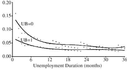
The crucial role of unemployment benefits in retarding transitions out of unem-ployment is now addressed in more detail. Hazard functions by destination state are charted in Figures 4 and 5. The estimates are again based on the defective risks model contained in the two final columns of Table 2. Note that the hazards in Figures 4 and 5 are unconditional, and use average values of the variables in their construc-tion; that is, they also reflect the presence of stayers on transition rates. Since the hazard functions depicted in the figures reflect the representation of a sub-population of individuals evincing zero escape rates, the effect will be to drive down the hazard rates and produce a tendency toward negative duration dependency because the sam-ple will comprise an increasing proportion of stayers with the passage of time. This effect also implies that the hazard functions will no longer be proportional to each other, even though they retain the proportionality property among movers.
For the employment cause-specific hazard function, there is a tendency for escape rates to fall with jobless duration for both recipients and nonrecipients alike. The
Figure 4
Cause-Specific Hazard Function—Employment
Addison and Portugal 179
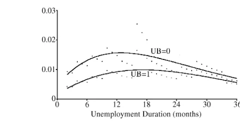
Figure 5
Cause-Specific Hazard Function—Inactivity
Note: Hazard function obtained from the specification in Table 2, Column 6. Hazard functions are unconditional, reflecting the presence of stayers.
decline for nonrecipients is fairly sharp over the first 12 to 18 months of the jobless spell, after which point the decline is modest, with a slight uptick after the 25th month. For recipients, the decline is both more muted and shorter lived. (Figure 7 makes the purely technical point that, if there were noU-I stayers, the employment cause-specific hazard function for nonrecipients would indicate a rise in escape rates a little after 12 months into the jobless spell. Although not presented graphically, the same result obtains for unemployment benefit recipients.)
Transitions into inactivity in Figure 5 display a quite different pattern. For both nonrecipients and recipients the hazard rises and then falls, peaking at around 12 months for the former and 18 months for the latter. As before, escape rates into inactivity are uniformly higher for nonrecipients than for recipients. While we have no cogent explanation for the shape of the hazard function, there is no real indication
Figure 6
Those Moving into Inactivity as a Proportion of all Transitions
Note: Computed as the ratio of the inactivity hazard function to the aggregate hazard function (the sum of the two specific hazard functions).
Figure 7
Nonrecipient Employment Hazard Function with and without Defective Risks
Note: Comparison of conditional (solely for U-E movers) and unconditional (aggregating movers and stayers) hazard functions.
Values obtained from the specification in Table 2, Column 5.
that transitions into inactivity are an end-state realized after fruitless search for em-ployment. Having said that, as can be seen from Figure 6, the proportion of transi-tions into inactivity does increase noticeably during the initial 12 months of unem-ployment. In this regard, differences between recipients and nonrecipients are muted, both functions peaking at a little less than 30 percent after 18 months.
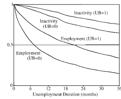
Aggregate survival functions and cause-specific survival functions for the two destination states are given in Figures 8 and 9, respectively. Both are computed from
Figure 8
Aggregate Survival Functions by UB Status
Note: Values obtained from the specification in Table 2, Columns 5 and 6.
Addison and Portugal 181
Figure 9
Specific Survival Functions by UB Status
Note: Values obtained from the specification in Table 2, Columns 5 and 6.
The ‘‘specific’’ survival functions converge to the proportion of stayers in each destination.
the last two columns of Table 2. That is, the aggregate survival function is simply obtained by the multiplication of the specific survivor functions given bySˆj
mabove. In short, the survivor rates are determined by both movers and stayers. From Figure 8 it can be seen that estimated median joblessness duration is around six months for nonrecipients and more than 16 months for recipients, and that defective risks apply. The aggregate survivor function in Figure 8 does not converge to zero. Rather, it converges to 0.106 (0.021) for unemployment benefit recipients (nonrecipients). These values denote the proportions of long-term unemployed. They are simply the product of the proportion ofU-E stayersandU-I stayers: 0.370⫻0.287 in the case of recipients and 0.091⫻0.231 for nonrecipients. Consistent with the information provided earlier on the cause-specific hazard functions, the disaggregated functions in Table 9 make it clear that survival rates for inactivity are much higher than for employment, and in each case higher for recipients than nonrecipients.
Our analysis also indicated that age is an important determinant of escape rates out of unemployment. Figures 10 and 11 reconsider the association between age and destination state (see also Table 3, below). The former figure indicates that the proportion ofU-E stayers—those who will never receive acceptable job offers— rises with age and in the same manner for recipients and nonrecipients alike. On the other hand, the latter figure demonstrates that the proportion ofU-1 stayersis de-creasing in age. Both effects are reinforcing in the unemployment duration of older workers.
Figure 10
Defective Risk into Employment by Age and UB Status
Note: Vertical axis gives the proportion of U-E stayers (non-employable) for individuals with mean characteristics for the continuous variables and reference category for the binary variables. Simulation values are obtained from the split-population equation estimates in Table 2, Column 5.
Figure 11
Defective Risk into Inactivity by Age and UB Status
Addison
and
Portugal
183
Table 3
Simulations from the Split-Population Model
Age⫽20 Years Age⫽35 Years Age⫽50 Years
UB⫽0 UB⫽1 UB⫽0 UB⫽1 UB⫽0 UB⫽1
Survival Rate after
3 months 0.629 0.792 0.672 0.841 0.790 0.920
12 months 0.257 0.466 0.321 0.574 0.474 0.723
36 months 0.050 0.140 0.092 0.250 0.218 0.435
Defective Risk
Employment 0.029 0.081 0.094 0.231 0.371 0.632
Inactivity 0.390 0.483 0.287 0.370 0.173 0.234
Median duration (in months)
Two destinations 5 11 7 16 11 28
Until employment 7 14 7 21 24 na
for recipients, but age is more important than access to benefits in arresting the decline in survival rates. Notice that this depressing effect of age on the intensity of transitions out of unemployment is mainly driven by the increase inU-E stayers
with age and not by the decrease in the hazard rates amongU-E movers. Similarly, although the pattern of survival rates at 3, 12, and 36 months points to greater persis-tence among recipients and older individuals, the increase in survival rates with age always exceeds the corresponding increase in survival rates with benefits. That being said, the impact of benefit receipt is profound; for example, at 36 months the survival rates of recipients are more than double those of nonrecipients for each of the three age groups.
The entries for defective risks (namely, eitherU-EorU-I stayers) show that the proportion of those who never get a job offer rises steadily with age and with benefit receipt by age. Roughly three (eight) percent of 20 year-old nonrecipients (recipients) will not receive an acceptable job offer, rising to 37 (63) percent in the case of their 50 year-old counterparts. The proportions of those who will never transition into inactivity declines with age and benefit receipt in roughly equal proportion (see also Figure 11).
The estimated median jobless duration values—shown at the foot of the table— while again confirming the important role of age and benefits in retarding transitions out of unemployment, make the point that destination state also matters. We present two sets of estimates of median duration. In one case, we admit—as is in practice the case—an individual can move into either employment or inactivity. This is con-sistent with a conventional interpretation and statistical definition of unemployment duration. In the other, we simulate a situation where the possibility of entering inac-tivity is precluded, and compute the length of time it will now take to find employ-ment if inactivity is ruled out, namely, the time needed to find a job. It can be seen that under the latter exclusion, duration would increase from 5 to 7 weeks for a 20 year old nonrecipient and from 11 to 14 weeks for his recipient counterpart. By the same token, duration would rise from 11 to 24 weeks for a 50 year-old nonrecipient.10 This type of simulation is straightforward in the framework of an independent com-peting risks model, where one can easily compute the duration for a given risk (or destination) precluding some or all the other risks. In this case, if inactivity is not possible, the duration of unemployment will be given simply by the U-Especific survival function.
V. Conclusions
It is important to underscore the point that defective risks are compat-ible with a variety of structural models of unemployment. Thus, for example, the hiring model of Blanchard and Diamond (1994), in which would-be employees are ranked by employers on the basis of their jobIess duration, implies latent infinite durations because some workers will never get hired. Defectiveness may also arise if individuals rule out certain destinations. The obvious analogy here is the
Addison and Portugal 185
firm matching model of Jovanovic (1979), in which some workers are so contented with their job match that they remain employed forever, leading to a defective tenure distribution. In the present paper, we used the organizing device of a polynomial distribution to effect a test of two such sources of defective risks: (a) a model of unlucky draws in which everyone is equally likely to end up permanently jobless, and (b) a model with separate populations of movers and stayers in which defectiveness is produced by the behavior of the latter. On this occasion, the split-population model won out.
Our split-population model provides a compelling explanation for European struc-tural unemployment and the interplay between inactivity and employment. It will be recalled that for individuals to be consigned to the unemployment state forever requires them to be defective in each of two transitions, namely, from unemployment to employment and from unemployment to inactivity. The permanently unemployed are thus the product of two probabilities. Our simulations confirmed that the product is nontrivial, especially when one considers subgroups of the population.
It is also important to emphasize that the likelihood of confronting defective risks increases with the number of destinations (that is, more states than just employment and inactivity). This possibility considerably extends the reach of this kind of model to a variety of research questions that involve duration analysis, and not solely the study of economies where long-term unemployment is the dominant policy concern. But assuredly, in the context of unemployment analysis, the more dramatic content of the model is likely to obtain in circumstances of protracted unemployment. To repeat, some individuals either as a result of their past choices or current endowments may be permanently jobless.
The statistical advantages of the split-population model are also worth emphasiz-ing. They are basically threefold. In the first place, if defective risks are present, it is obvious that traditional approaches will lead to inconsistent estimates of the hazard regression coefficients. Indeed, it was shown that some regression coefficient esti-mates—for example, the age coefficients—changed dramatically after taking the presence of stayers into account. In the second place, the shape of the baseline hazard function will be misspecified, biasing the parameter estimates toward negative dura-tion dependence because the relative propordura-tion of stayers increases with time. Fi-nally, and no less important, the model allows us to straightforwardly identify factors that influence the presence of stayers. These advantages are achieved at no significant cost because conventional unemployment duration models are special cases of this mover-stayer treatment. Despite its heavy parameterization, the computational bur-den of estimating the split-population model was surprisingly light. Moreover, the results obtained were plausible and obtained with fairly good precision.
permanently unemployed—up to 13.7 percent (5.2 percent) of 50 year-old UI recipi-ents (nonrecipirecipi-ents)—is a worrying finding of our analysis. Further study of this issue is urgently required, using structural approaches to investigate whether it is a reservation wage phenomenon or rather, as we suspect, a function of the arrival rate of job offers. As far as unemployment benefits are concerned, their negative effect in slowing transitions out of unemployment and increasing the proportion of long-term unemployed is massive. The effects of age and access to benefits in increasing the proportion of those who will never find work were found to be reinforcing. This conjunction would appear to question the logic of making maximum potential dura-tion of benefits so heavily dependent upon age (or previous tenure, as is widely the case in Europe). There is another issue for policy: if the costs of unemployment are so dramatic for workers (in terms of jobless duration), and firms do not internalize these costs, then a strong case can be made for the introduction of experience rat-ing as a partial offset. Finally, we note that the familiar pro-supply effect of marital status is confirmed in our analysis: being married increases (decreases) the employ-ment (inactivity) hazard and reduces the proportion of both types of stayers (namely,
Addison
and
Portugal
[image:32.612.131.658.207.409.2]187
Table A1
Definition of Variables and Sample Means by Unemployment Benefit Recipiency and Destination
Recipient Nonrecipient
Variable Unemployed Employed Inactive Unemployed Employed Inactive
Duration (elapsed unemployment in months) 12.082 9.027 15.250 16.138 9.919 13.548
Age (age in years) 42.456 36.048 43.875 31.184 29.457 30.158
Schooling (years of schooling completed) 5.765 5.912 5.312 7.089 7.104 7.743
Tenure (years of tenure on previous job) 10.221 5.739 11.775 4.159 2.749 4.215
Jobs (number of previous jobs) 3.431 3.958 3.250 2.419 3.011 1.892
Married (⫽1 if married, 0 otherwise) 0.754 0.636 0.734 0.338 0.369 0.278
First job (⫽1 if looking for first job, 0 otherwise) 0.234 0.174 0.361
Layoff (⫽1 if job lost by reason of mass layoff, 0.316 0.227 0.203 0.093 0.082 0.046
0 otherwise)
End fixed (⫽1 if job lost by termination of a 0.243 0.382 0.266 0.244 0.332 0.174
fixed-term contract, 0 otherwise)
Unemployment rate (quarterly unemployment rate) 6.648 6.570 6.684 6.557 6.498 6.388
The
Journal
of
Human
[image:33.612.135.667.208.480.2]Resources
Table A2
Hazard Regression Model with Discrete Change After Six Months of Unemployment (n⫽9,451)
Polynomial Specification Piecewise-Constant Specification
Transition to Employment Transition to Inactivity Transition to Employment Transition to Inactivity
Change after Change after Change after Change after
Variable Durationⱕ6 Duration⬎6 Durationⱕ6 Duration⬎6 Durationⱕ6 Duration⬎6 Durationⱕ6 Duration⬎6
UB ⫺0.577 ⫺0.261 ⫺0.825 ⫺0.391 ⫺0.700 0.340 ⫺0.768 0.403
(0.107) (0.153) (0.406) (0.401) (0.145) (0.217) (0.503) (0.421)
Age group
25–29 0.119 ⫺0.261 ⫺0.597 0.199 0.201 ⫺0.217 ⫺0.640 0.390
(0.104) (0.170) (0.346) (0.487) (0.142) (0.255) (0.364) (0.550)
20–34 0.025 ⫺0.378 ⫺1.037 0.030 0.155 ⫺0.390 ⫺1.127 ⫺0.052
(0.129) (0.214) (0.553) (0.660) (0.177) (0.299) (0.591) (0.741)
35–39 ⫺0.078 ⫺0.470 ⫺0.388 ⫺0.781 0.199 ⫺0.370 ⫺0.511 ⫺1.324
(0.163) (0.280) (0.583) (0.764) (0.290) (0.357) (0.617) (0.854)
40–44 0.164 ⫺0.513 0.028 ⫺0.295 0.520 ⫺0.712 ⫺0.125 ⫺0.102
(0.162) (0.284) (0.639) (0.740) (0.243) (0.408) (0.671) (0.819)
45–49 0.062 ⫺0.510 0.013 ⫺0.619 0.324 ⫺0.926 ⫺0.281 ⫺0.750
(0.190) (0.325) (0.677) (0.790) (0.263) (0.458) (0.765) (0.889)
50–54 0.043 ⫺0.733 0.160 ⫺0.279 0.445 ⫺1.119 ⫺0.263 ⫺0.540
(0.236) (0.379) (0.734) (0.789) (0.331) (0.530) (0.773) (0.866)
55⫹ ⫺0.207 ⫺0.802 ⫺0.526 0.493 0.144 ⫺1.315 ⫺0.912 0.527
(0.252) (0.441) (0.756) (0.812) (0.334) (0.557) (0.924) (0.918)
Schooling 0.006 0.023 ⫺0.035 ⫺0.022 0.015 ⫺0.004 ⫺0.068 ⫺0.025
(0.011) (0.019) (0.046) (0.052) (0.016) (0.026) (0.050) (0.058)
Tenure ⫺0.026 0.022 0.012 ⫺0.002 ⫺0.028 0.015 ⫺0.005 ⫺0.005
Addison
and
Portugal
189
Married 0.152 0.331 ⫺1.404 0.870 ⫺0.002 0.219 ⫺0.753 0.865
(0.108) (0.197) (0.531) (0.556) (0.148) (0.252) (0.602) (0.601)
First job ⫺0.476 0.067 0.485 0.210 ⫺0.612 0.399 0.501 ⫺0.071
(0.126) (0.191) (0.283) (0.445) (0.164) (0.280) (0.331) (0.512)
Layoff ⫺0.121 0.198 ⫺0.611 ⫺0.245 ⫺0.124 0.021 ⫺0.549 ⫺0.456
(0.138) (0.203) (0.518) (0.597) (0.169) (0.253) (0.527) (0.627)
End fixed 0.097 0.207 ⫺0.205 ⫺0.275 0.161 ⫺0.122 ⫺0.056 ⫺0.561
(0.080) (0.148) (0.276) (0.388) (0.011) (0.194) (0.303) (0.450)
Unemployment rate ⫺0.056 0.152 ⫺0.532 0.437 ⫺0.071 0.185 ⫺0.446 0.465
(0.035) (0.066) (0.133) (0.158) (0.050) (0.095) (0.162) (0.170)
Sigma 0.177 0.410 0.599 0a
(0.427) (0.670) (0.162)
Split-population equation
Mu 5.170 0.683 1.963 0.413
(1.377) (0.522) (0.198) (0.359)
UB ⫺1.390 ⫺0.134 ⫺0.733 ⫺0.150
(0.580) (0.861) (0.280) (0.728)
Age ⫺0.170 0.032 ⫺0.090 0.033
(0.050) (0.032) (0.013) (0.022)
Schooling ⫺0.127 0.211 ⫺0.039 0.185
(0.058) (0.078) (0.029) (0.060)
Tenure ⫺0.037 ⫺0.022 ⫺0.030 0.021
(0.022) (0.038) (0.013) (0.022)
Married 1.024 2.584 1.389 0.040
(0.867) (1.362) (0.282) (0.657)
Unemployment rate ⫺0.540 0.352 ⫺0.053 0.121
(0.490) (0.183) (0.132) (0.165)
Log-likelihood ⫺5,001.89 ⫺5,041.5
Note: Asymptotic standard errors in parentheses.
References
Addison, John T., and Pedro Portugal. 2002. ‘‘Job Search Methods and Outcomes.’’
Ox-ford Economic Papers54(3):505–33.
Blanchard, Olivier, and Peter Diamond. 1994. ‘‘Ranking, Unemployment Duration, and
Wages.’’Review of Economic Studies61(3):417–34.
Blanchard, Olivier, and Pedro Portugal. 2001. ‘‘What Hides Behind an Unemployment
Rate: Comparing Portuguese and U.S. Labor Markets.’’American Economic Review
91(l):187–207.
Bover, Olympia, Pilar Garcı´a-Perea, and Pedro Portugal. 2000. ‘‘Labour Market Outliers:
Lessons from Portugal and Spain.’’Economic Policy15(31):381–428.
Cockx, Bart L. W. 1997. ‘‘Analysis of Transition Data by Minimum-Chi Square Method:
An Application to Welfare Spells in Belgium.’’Review of Economics and Statistics
79(3):392–405.
Cox, D.R., and D. Oakes. 1985.Analysis of Survival Data. London: Chapman and Hall.
Crowder, Martin. 2001.Classical Competing Risks. New York: Chapman & Hall.
Fallick, Bruce Chelimsky. 1991. ‘‘Unemployment Insurance and the Reemployment Rate
of Displaced Workers.’’Review of Economics and Statistics73(2):228–35.
Flinn, Christopher J. 1986. ‘‘The Econometric Analysis of CPS-Type Unemployment
Data.’’Journal of Human Resources21(4):456–89.
Flinn, Christopher J., and James J. Heckman. 1982. ‘‘Models for the Analysis of Labor
Force Dynamics.’’ InAdvances in Econometrics, Vol. 1, ed. R. L. Basmann and G. F.
Rhodes, 35–95. Greenwich, Conn.: JAI Press.
———. 1983. ‘‘Are Unemployment and Out of the Labor Force Behaviorally Distinct
La-bor Market States?’’Journal of Labor Economics1(1):28–42.
Han, A., and J. Hausman. 1990. ‘‘Flexible Parametric Estimation of Duration and
Compet-ing Risks Models.’’Journal of Applied Econometrics5(1):1–28.
Heckman, James J., and Burton Singer. 1985. ‘‘Social Science Duration Analysis.’’ In
Lon-gitudinal Analysis of Labor Market Data, ed. James J. Heckman and Burton Singer, 39– 58. Cambridge: Cambridge University Press.
Heckman, James J., and Bo Honore´. 1989. ‘‘The Identifiability of the Competing Risks
Model.’’Biometrika76:325–30.
Heckman, James J., and James R. Walker. 1990. ‘‘Estimating Fecundability From Data on
Waiting Times to First Conception.’’Journal of American Statistical Association
85(410):83–94.
Ibrahim, Joseph, Ming-Hui Chen, and Debajyoti Sinha. 2001.Bayesian Survival Analysis.
New York: Springer-Verlag.
Jovanovic, Boyan. 1979. ‘‘Job Matching and the Theory of Turnover.’’Journal of
Politi-cal Economy87(5):972–90.
Kalbfleisch, J. D., and R. L. Prentice. 1980.The Statistical Analysis of Failure Time Data.
New York: Wiley.
Lancaster, Tony. 1990.The Econometric Analysis of Transition Data. Cambridge:
Cam-bridge University Press.
Maller, Ross, and Xian Zhou. 1996.Survival Analysis with Long-Term Survivors.
Chiches-ter and New York: John Wiley and Sons.
McLachlan, Geoffrey, and David Peel. 2000.Finite Mixture Models. New York: John
Wi-ley & Sons, Inc.
Addison and Portugal 191
Meyer, Bruce D. 1990. ‘‘Unemployment Insurance and Unemployment Spells.’’
Economet-rica58(4):757–82.
Narendranathan, Wiji, and Mark B. Stewart. 1993. ‘‘Modeling the Probability of Leaving
Unemployment: Competing Risks Models with Flexible Base-Line Hazards.’’Applied
Statistics—Journal of the Royal Statistical Society Series C42(l):63–83.
OECD. 1999.Employment Outlook, Paris: Organisation for Economic Co-operation and
De-velopment.
Portugal, Pedro, and John T. Addison. 1995. ‘‘Short- and Long-Term Unemployment. A
Parametric Model with Time-Varying Effects.’’Oxford Bulletin of Economics and
Statis-tics57(2):205–27.
Pudney, Stephen, and Jonathan Thomas. 1995. ‘‘Specificati