Cognitive Development
Christopher J. Ruhm
a b s t r a c t
Maternal employment during the rst three years of the child’s life has a small deleterious effect on estimated verbal ability of three- and four-year-olds and a larger negative impact on reading and mathematics achievement of ve- and six-year-olds. This study provides a more pessi-mistic assessment than most prior research for two reasons. First, previ-ous analyses often control crudely for differences in child and hprevi-ousehold characteristics. Second, the negative relationships are more pronounced for the reading and mathematics performance of ve- and six-year-old children than for the verbal scores of three- and four-year-olds.
I. Introduction
The rst three years of life are a particularly important period for children (Carnegie Task Force on Meeting the Needs of Young Children 1994; Coun-cil of Economic Advisers 1997). Recent research emphasizes the effects of early inuences on brain development (Shore 1997) and investments by parents during
Christopher J. Ruhm is a professor of economics at the University of North Carolina at Greensboro and a research associate at the National Bureau of Economic Research. He thanks Carey Borkoski for research assistance and Li Gan, Hilary Hoynes, Dan Rosenbaum, Donna Ruane Morrison, David Wildesin, and seminar participants at Case Western Reserve University, Georgetown University, the In-stitute for the Study of Labor, University of California at Berkeley, University of Kentucky, University of Texas, University of Virginia, University of Washington, and Vanderbilt University for helpful com-ments. Financial support from the University of North Carolina Greensboro, the National Science Foundation (SES-9876511), and the National Institute of Child Health and Human Development (HD38521-01A1) is gratefully acknowledged. All opinions, ndings, and conclusions or recommenda-tions are those of the author and do not necessarily reect the views of the funding agencies. The data used in this article can be obtained beginning August 2004 through July 2007 from Ruhm.
[Submitted June 2001; accepted September 2002]
ISSN 022-166XÓ2004 by the Board of Regents of the University of Wisconsin System
early childhood are likely to be signicant for the development of learning skills, self-esteem, and emotional security (Heckman 2000).1
Between 1980 and 1998, the labor force participation rate of mothers with children six years old and younger grew from 47 to 65 percent (U.S. Department of Com-merce 1999). The increase was even larger for women with infants, rising from 38 to 59 percent (Bachu and O’Connell 2000). These changes, when combined with the growth in single-parent households, suggest that adults have less time and energy to invest in their offspring, with potentially deleterious effects.2However, increased market work may also yield benets, most obviously by providing extra income.
This paper analyzes the relationship between parental employment and three high quality assessments of the cognitive skills of young children. Data are from multiple years of the National Longitudinal Survey of Youth (NLSY). The results suggest a deleterious effect of early maternal employment. Working during the rst year is associated with reductions in the verbal ability of three- and four-year-olds that are partially (but not completely) offset by increases from job-holding during the next two years. Employment in the rst three years is more strongly negatively related to the reading and mathematics achievement of ve- and six-year-olds and labor supply in the child’s second and third year is estimated to have more harmful (or less favorable) consequences when the mother works long hours or also held a job in the rst year. The data also hint at the importance of time investments by fathers, although this analysis is preliminary.
These ndings contrast with previous research indicating positive or neutral effects of parental employment during the rst three years and recent studies identifying deleterious impacts of working during infancy but not thereafter. There are two main reasons for the more pessimistic results. First, the negative relationships are stronger for the reading or mathematics achievement of ve- and six-year-olds than for the more commonly examined verbal ability of three- and four-year-olds. Second, chil-dren with working parents come from relatively advantaged family backgrounds and possess attributes that promote cognitive development. Most prior analyses inade-quately control for this heterogeneity and therefore substantially understate the costs of early employment. This study does a better job of accounting for the disparities and so provides a less favorable assessment. However, to the extent that all confound-ing factors are still not held constant, these estimates may continue to provide biased estimates, highlighting the need for further research.
II. Previous Research
The relationship between early maternal employment and child cog-nitive development has been widely studied. A few investigations nd positive
ef-1. However, the mechanisms for these effects are poorly understood and the relationship between early brain development and future outcomes remains controversial (Bruer 1999).
fects (Vandell and Ramanan 1992; Parcel and Menaghan 1994; Moore and Driscoll 1997), others negative impacts (Leibowitz 1977; Stafford 1987; Mott 1991), and many obtain results that differ depending on the timing of work or the specic group analyzed (Desai, Chase-Lansdale, and Michael 1989; Baydar and Brooks-Gunn 1991; Blau and Grossberg 1992; Parcel and Menaghan 1994; Greenstein 1995).3
A common conclusion of the most recent (and generally carefully conducted) analyses is that maternal employment during the child’s rst year has a deleterious impact (James-Burdumy 1999; Neidell 2000; Han, Waldfogel and Brooks-Gunn 2001; Hill et al. 2001; Brooks-Gunn, Han and Waldfogel 2002; Waldfogel, Han, and Brooks-Gunn 2002) but often with no effect or offsetting benets for working during the second and third year.4Harvey (1999) nds that the negative impact of rst year employment is temporary, whereas Han, Waldfogel, and Brooks-Gunn (2001) and Waldfogel, Han, and Brooks-Gunn (2002) indicate greater persistence. The patterns may also vary with factors such as race, sex of the child, household structure, and family income in ways that are poorly understood. The limited research on paternal employment obtains inconclusive results (Parcel and Menaghan 1994; Harvey 1999; Ermisch and Francesconi 2001; Waldfogel, Han, and Brooks-Gunn, 2002).
These inferences should be viewed as tentative because parents holding jobs or working long hours may differ from those who do not in ways that have been inade-quately accounted for. Mothers with characteristics associated with high ability, such as education levels and AFQT scores, tend to have elevated employment rates (Van-dell and Ramanan 1992; Hill et al. 2001; Waldfogel, Han, and Brooks-Gunn 2002). If these advantages extend to productivity in home activities, maternal employment will be positively associated with child outcomes, even absent a causal impact.5 Without an exogenous source of variation in labor supply, it is difcult to completely eliminate potential omitted variables bias. The primary approach below is to include an unusually comprehensive set of explanatory variables and to examine how the
and Hofferth (2001) argue that behavioral changes by parents have prevented any decrease in the time actually devoted to children since the early 1980s.
3. Related research examining if early childcare harms infant-mother attachments (Belsky and Rovine 1988; Clarke-Stewart 1989; Lamb and Sternberg 1990; NICHD Early Child Care Research Network 1997b) suggests that maternal employment, by increasing the use of day care, could reduce attachment security in some situations. However, the size and pattern of the effect is uncertain and none of the studies use nationally representative samples or sufciently control for parental abilities or attitudes.
estimates change when sequentially accounting for an increasing portion of the het-erogeneity. The addition of more complete controls reduces (increases) the estimated benets (costs) of early employment. This suggests that previous investigations may present an overly optimistic assessment.
III. Conceptual Framework
Economic models portray households as productive entities where parents allocate resources to maximize an objective function that includes the health and development of children as one argument. Holding marital status and household size constant, more time, energy, and income are likely to be devoted to children as more of each are available to the parents.6Parental employment may therefore improve child outcomes by increasing incomes. However, under general conditions, market employment is also likely to lead to at least some decrease in child-related investments in time or energy. Time-diary data conrm that working mothers spend less time with children than do their nonemployed counterparts (Bryan and Zick 1996; Zick and Bryan 1996; Bianchi 2000; Gershuny 2000; Hofferth 2001; Sandberg and Hofferth 2001), although there is considerable uncertainty about the size of this effect.7 Long hours might also cause parents to be tired or stressed, reducing the quality of the time with children.8
The psychological and sociological literatures emphasize complementary path-ways through which market work by parents may negatively affect child develop-ment. Belsky (1988) argues that a mother’s absence during the rst year of life could disrupt mother-child attachments and deprive the child of the stimulation that promotes cognitive development. Hoffman (1980) states that the stress of maternal employment may yield fewer and lower quality interactions. Coleman (1988) ex-presses concern that the job-holding will weaken the “social capital” that depends on the relationships in which children are embedded. These effects may also vary with household characteristics and age of the child. If well-off parents provide higher quality time, for instance, employment could be more harmful in rich than poor families. Conversely, wealthier families can afford better daycare and educated
6. Leibowitz (1974a) provides early research highlighting parental time investments in children. There is wide agreement that children benet from being in households with higher incomes but debate over the nature of the relationship. Duncan and Brooks-Gunn (1997) emphasize the causal effect of poverty, whereas Mayer (1997) suggests weaker income effects, possibly because a greater portion of family income is devoted to children in poor than wealthy families (Lazear and Michael 1988). All else equal, more time will also be invested in children with fewer siblings and in two-parent (versus single-parent) households (Haveman and Wolfe 1995; McLanahan 1997).
7. Employed females may “protect” the most productive time by cutting back least on activities that di-rectly engage children. Increased time investments by fathers could offset the reductions of working moth-ers (in two family households) but little empirical evidence supporting this possibility has been provided. The involvement of fathers in child care is rising over time (Bianchi 2000) but paternal labor supply is unrelated or negatively related to the hours fathers spend with children (Gershuny 2000; Hofferth 2001). This last issue receives attention in the analysis of paternal employment below.
women spend a greater proportion of their nonmarket time in child-related activities (Leibowitz 1974b).9
These approaches all stress the benecial effects of household income and direct parental investments in children, suggesting a potential tradeoff between the two. To illustrate, consider a production function where child outcomes at age t (Ct) depend on status in the previous period (Ct21), the nonmarket “leisure” time of parents (L), purchased inputs like food or medical care (F), and exogenous determi-nants or production shocks (V) according to:
(1) Ct5C(Ct21,Lt,Ft,Vt).10
Using subscripts to indicate partial derivatives,CLandCFare positive. The produc-tion funcproduc-tion has several important characteristics. First, parental leisure is good for children. This occurs either through direct time investments or indirectly through reductions in stress, increased energy levels, and so forth. Second, higher incomes raise the ability of parents to purchase productive inputs and inuence their time allocation decisions. Third, child outcomes depend partly on prior status and there-fore on endowments and the past choices of parents.
Parents have a time constraint (2) Lt1Ht51,
whereHandLare the proportions of total time spent in employment and nonmarket activities.11The household also has a budget constraint that limits purchases of child inputs and other consumption to the amount of earned and nonearned income. Solv-ing Equation 2 for Hand recursively substituting in for lags ofC, Equation 1 can be rewritten as:
(1¢) Ct 5C(H,F,V),
whereH,F, andVare vectors of current and lagged values (for instance,H5{Ht, Ht21, . . .Ht2n}, fort2nthe rst period where parental inputs affect child outcomes). MaximizingC subject to income and time constraints yields the reduced-form de-mand function:
(3) Ct5C(P,V),
wherePis a vector of current and lagged prices and wages.12
Estimates of the child production or reduced-form demand functions specied by Equations 1¢ or 3 provide policy-relevant parameters of structural determinants of child development. However, data restrictions preclude the estimation of either
9. The average quality of child care increases with income, although center-based care for low-income children appears to be of relatively high quality (NICHD Early Child Care Research Network 1997a), probably due to early intervention programs (such as Head Start) that are available to poor families. 10. This model follows Becker (1981) in emphasizing the role of nonmarket time in household production and Grossman (1972) in treating health as an outcome produced by investment activities.
model, since information is lacking on the full vector of relevant prices and many individual-specic production shocks. Instead, this analysis focuses on what Rosen-zweig and Schultz (1983) refer to as “hybrid” equations. These take the form: (4) Ct5C(H,X,e),
where Hmeasures work hours, X is a vector of individual or family background characteristics, ande is a disturbance term capturing production shifters or shocks not otherwise controlled for.
A limitation of the hybrid equations is that the coefcient estimates generally embody both the technological properties of the production function and the charac-teristics of unobserved household preferences or production shifters. For example, the proportion of total income devoted to children may vary with family background characteristics, and parental attitudes about labor supply could be correlated with other investments in children. Child outcomes similarly depend on the quality as well as thequantityof parental time, and the “technologies” in place when decisions are made. For instance, since child care is one purchased input, the effects of employ-ment partly depend on the difference in the quality of parental and nonparental care. One result is that any negative effects of labor supply are likely to rise as the price-adjusted quality of day care falls.13A fully specied model would account for the endogeneity between these technologies and parental decisions but the regression estimates below do not. Instead, the employment coefcients indicate the “effects” of working given the average differences in other factors (such as child care) that accompany the variation in labor supply. An implication is that limited information is provided on how parental employment will affect child development in different institutional environments, such as those in many European nations.14
Moreover, a causal interpretation can only be applied to the parameter estimates on parental employment if the variables inXcapture the effects of all other structural determinants of child outcomes. A particular concern is the difculty in adequately controlling for heterogeneity in family or child characteristics correlated with paren-tal job-holding. This represents a major challenge for all related research in this area.
IV. Econometric Issues
The model above is operationalized by assuming that the cognitive assessment score for childiat aget (Cit) is an additive separable function of parental work hours at child agestthrough t2n (Hit 5{Hit,Hit21, . . .Hit2n}) and other production shifters (Vit), according to:
(5) Cit5a1Hitbt1Vit1eit,
for eit an i.i.d. disturbance.15Implicit in Equation 5 is the assumption that parental job-holding prior tot2nor after thas no impact on child outcomes at aget. For this analysis, I assume thatt2nis the period immediately following birth.16
Several important econometric issues can be claried using an even simpler (but unrealistic) model where only contemporaneous employment affects child outcomes (Hit5{Hit}). In the absence of additional controls, this implies the regression equa-tion:
(6) Cit5a1Hitb1eit,
whereeit5Vit 1eit.bˆ is then biased if cov(Hit,eit)¹0, which occurs ifVis correlated with H. For example, there is a spurious positive relationship if employed women have high home productivity or their children have endowments associated with high levels of cognitive skill.
The primary econometric strategy is to use the detailed information in the NLSY to directly account for many potential confounding factors. Thus,
(7) Cit5a1Hitb1Xitg1mit,
consistently estimates the effects of parental employment if the supplementary re-gressors (X) control for other determinants of child development, such that cov(Xit, mit)5 cov(Hit,mit)50. The goal therefore is to include a sufciently rich set of covariates that the error term is orthogonal toHit. However, it is important to exclude variables thatresultfrom parental job-holding (such as the home environment during the child’s early years), since these capture a portion of the labor supply effect. An exception is that some models hold constant family income or the use of nonparental child care, both of which are likely to be affected by work hours, to examine the extent that the impact of parental employment operates through these factors.
Most models also control for maternal employment after the child’s third year. This has rarely been done in prior research, with the result that the previously esti-mated effects are likely to combine the impact of working during the rst three years with those of labor supply in later periods. To illustrate, consider the situation where Hit5{Hit,Hit21}, fortthe assessment year andt21 the early childhood period of interest. Further assume that regressions of:
(8) Cit5a1Hit21bt211Hitbt1Xitg1mit yield unbiased estimates. If the model used is (8¢) Cit 5a1Hit21bt211Xitg1lit,
wherelit5Hitbt1mit, cov(Hit21,git)5btcov(Hit21,Hit) andbˆt21is biased in the direction of btif employment is positively correlated over time.17
Even an extensive set of explanatory variables may not fully account for all
impor-15. The model could be modied to include lags of the production shifters.
16. This assumption could be violated if, for example, intertemporal nancial transfers cause work before birth to raise consumption during the child’s early years.
tant sources of heterogeneity. However, under reasonable assumptions, employment prior to birth can be added to the regression equation to test for bias due to unob-served maternal factors.18To see this, rewrite the model in Equation 7 as: (7¢) Cijt5a 1Hijtb1Xijtg1mijt,
where j subscripts the child’s mother. Decompose the error term as mijt 5 Mj 1 Ki1jijt, whereMare time-invariant maternal characteristics,K are child-specic endowments that are orthogonal to maternal factors (implying that cov(Mj,Ki)50), andjis an i.i.d. error.19AllowHto be related toMandKaccording to:
(9) Hijt5CtMj 1dtKi1pijt. Ifpis an i.i.d. disturbance,
(10) cov(Cijt,Hijt)5bvar (Hijt)1ctvar(Mj)1dtvar (Ki).
The last two terms in Equation 10 therefore indicate the biases from failing to control for omitted maternal and child effects.
Assuming that work in the year prior to birth (Hijt2p) does not inuence child outcomes and is unaffected by endowments of the (as yet unborn) child,
(11) cov(Cijt,Hijt2p|Hijt)5ct2pvar (Mj)
anddˆ provides an estimate of the heterogeneity bias due to the mother-specic effects in the augmented regression model
(12) Cijt5a1Hijtb1Xijtg1Hijt2pd1mijt.
In particular, ifct5ct2p,dˆ50 indicates that this source heterogeneity is completely accounted for.
This procedure will generallynot test for bias due to unobserved child-specic factors. This may be even more of an issue in research using maternal xed-effects (James-Burdumy 1999; Neidell 2000; Ermisch and Francesconi 2001; Waldfogel, Han, and Brooks-Gunn, 2002) to control for heterogeneity in family backgrounds. The xed-effect (FE) models correspond to:
(13) Cijt5a1Hijtb1Xijtg1Mjd1fijt,
whereMis a vector of mother-specic dummy variables andfijt5Ki1jijt. Such specications exploit intra-family variations, as can be seen by representing sibling disparities in cognitive scores, maternal employment (at given child ages), and per-sonal characteristics using DC, DH, andDX and differencing Equation 13 within families to obtain:
(14) DCit5DHitb1DXitg1Dfit.
Notice that the maternal xed-effect has been eliminated. However, child-specic endowments have not and there is no reason to believe the FE models provide
consis-18. This approach draws heavily on the method used by Gottschalk (1996) for examining the intergenera-tional correlation in welfare participation.
tent estimates or even reduce the bias. Specically, since the error term in Equation 14 is Dfit 5DKi1Dfit, bias remains if cov(DHi,DKi)¹0 and may belarger than in corresponding OLS models if unobserved child-specic factors are a key determi-nant of sibling differences in maternal labor supply.20This is important because of evidence that mothers work less when children have health or developmental prob-lems.21This suggests that cov(DH
it,DKi).0 and that the FE models are likely to understate the costs or overestimate the benets of maternal employment.22
V. Data and Descriptive Results
Data are from the National Longitudinal Survey of Youth, a sample of U.S. residents born between January 1, 1957 and December 31, 1964 who have been surveyed since 1979.23In 1982 the NLSY began including questions on preg-nancy, prenatal, and post-natal care. Children born to and living with female NLSY respondents have been interviewed at two-year intervals beginning in 1986, with information used below through 1996. The combined data set provides a unique source of longitudinal information on a large sample of children and their parents, including great detail on maternal, child, and household characteristics.
The NLSY (through 1996) includes children whose mothers were aged 29 to 38 at the end of 1995. This covers approximately 80 percent of childbearing for this cohort but does not represent all fertility, since the offspring of some older women (who tend to have high incomes and education levels) are excluded. Although this selection should be kept in mind when interpreting the results, the sample ismore representative than that in most previous studies.
Cognitive development is proxied by scores on the Peabody Picture Vocabulary Test (PPVT) and the Peabody Individual Achievement Test Reading Recognition (PIAT-R) and Mathematics (PIAT-M) subtests.24These are among the most widely used assessments of preschool and early school-aged children and are known to have high test-retest reliability and concurrent validity (Baker et al. 1993). The PPVT measures receptive vocabulary for Standard American English and provides a quick estimate of verbal ability and scholastic aptitude. The PIAT-R indicates word recog-nition and pronunciation ability by examining skills such as matching letters, naming
20. The xed-effect models also use a less representative sample that is restricted to siblings in the age groups where complete data are available.
21. Low birthweight and slow developmental abilities delay the return of mothers to work (Neidell 2000). Employment is reduced if children have limiting health conditions or disabilities (Ermisch and Francesconi (2001). Mothers of “high risk” children return to jobs relatively slowly and parental employment is de-creased when children have low development scores or high levels of “fearfulness” Norberg (1998). Parents supply more (fewer) resources to siblings with lesser (greater) genetic endowments than if they were indifferent to the distribution of outcomes across children (Behrman, Pollack, and Taubman 1982). 22. However, debate on the preferred estimation method will continue until we better understand the processes linking parental employment to child outcomes.
23. The NLSY originally included a representative sample of 6,111 youths, an oversample of 5,295 blacks, Hispanics and economically disadvantaged whites, and a supplemental sample of 1,280 persons in the military in September 1978. Interviews with the military subsample were suspended after 1984 and for economically disadvantaged non-Hispanic whites after 1990. This data set is now sometimes referred to as the NLSY79, to distinguish it from the new NLSY97 survey which covers a later cohort.
names, and reading single words aloud. The PIAT-M assesses attainment in mathe-matics beginning with early skills, such as recognizing numerals, and progressing to advanced concepts in geometry and trigonometry.
The PPVT was administered to children aged three and older in 1986, with addi-tional assessments for previously untested age-eligible children in 1988, 1990, 1992, 1994, and 1996.25This investigation examines results for three- and four-year-olds. The PIAT-M and PIAT-R were given to children ve and older in each survey year, with data on ve- and six-year-olds used below.26The analysis focuses on “standard” assessment scores. These represent transformations, on an age-specic basis, of the raw scores that were originally (during the 1970s) designed to have a normal distribu-tion with a mean of 100 and a standard deviadistribu-tion of 15. Standard scores have been commonly used by previous researchers (Baydar and Brooks-Gunn 1991; Blau and Grossberg 1992, Parcel and Menaghan 1994). Models are also estimated using raw or percentile scores to ensure that the results are not sensitive to this choice.27For ease of interpretation, the dependent variables have been normalized to have a standard deviation of one. The regression coefcients therefore show the standard deviation change in the test score predicted by a one unit change in the explanatory variable. Maternal employment is measured in the year prior to birth (denoted as year zero) and in the rst through fourth years of the child’s life (Years 1 through 4). Most regressions control for average weekly work hours divided by 20.28 A one-unit change thus corresponds to switching from no employment to half-time work or from 20 to 40 hours per week on the job. To check the robustness of these results, some models instead control for: the proportion of weeks worked (multiplied by two), whether the mother held any job during the specied period, or the number of weeks after birth until she resumes employment.29
The NLSY contains limited information on fathers. One restriction is that data are only available for those residing with interviewed mothers. Therefore, the analysis of paternal employment is limited to (a potentially unrepresentative sample of) children with fathers in the household at the interview date of the fourth calendar year after birth. This is done because these men are likely to have been with the child through-out the rst three years. Data for thecalendar yearpreceding the survey date provide information on average weekly employment hours or the proportion of weeks worked
25. All age-eligible children were assessed in 1992, even if they had previously been tested.
26. Reading comprehension is also assessed for children receiving sufciently high PIAT-R scores. How-ever, this test rarely provides useful information for children younger than seven and is not utilized here. 27. The percentile scores are derived from the standard scores and represent a uniformly-distributed rank-ing of individuals in the original age-normed distribution. The raw scores are closer to a log-normal distri-bution, particularly for the PIAT-R and PIAT-M assessments. One implication, compared to the standard scores, the percentile scores will tend to place more weight on observations in the middle of the distribution and raw scores on those at its upper-tail.
28. Work hours cover all jobs held by the respondent. However, hours are calculated using data for the main job only in the few cases where information on secondary jobs is missing. NLSY mothers with a job but on maternity leave are generally categorized as employed; implying that employment rates immedi-ately after birth are overstated and the effects of maternal work during this period may be underestimated. However, few women are on maternity leave for more than a few weeks so the resulting bias is likely to be small. For instance, Klerman and Leibowitz (1994) nd that just 2.2 percent of mothers were on paid leave and 6.0 percent on unpaid leave three months after giving birth during the late 1980s.
by fathers.30For children born before (on or after) July 1, Year 1 refers to the calendar year of birth (the next calendar year). Thus, Year 1 includes the majority of the child’s rst year of life. Years zero, two, three, and four are dened in reference to Year 1.31
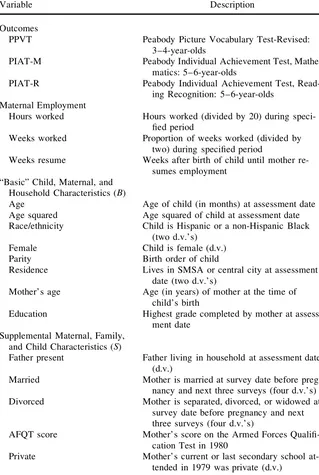
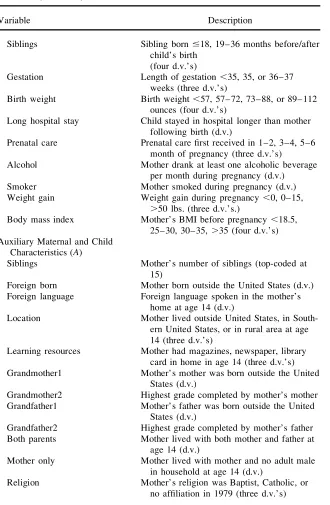
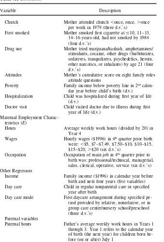
This analysis exploits the extensive child, maternal, and household information available in the NLSY. A vector of “basic” background variables, so labeled because they have frequently been used in previous research, contains continuous measures of birth order, mother’s age (in years) at child birth, her highest grade completed, and a quadratic for child age in months. Also included are dummy variables for race/ ethnicity (two variables), residence in an SMSA or central city (two variables), and sex of the child. Unless noted, all regressors are measured at the child assessment date. Appendix Table A1 provides detailed descriptions of all variables used in the analysis.
Most models also control for a set of “supplemental” characteristics. These include the mother’s Armed Forces Qualications Test (AFQT) score and marital status at the survey date before pregnancy and the next three surveys (eight variables), some form of which have occasionally been held constant in prior research. The vector also contains a family factors that may proxy determinants of child development but have not previously been controlled for, such as whether the mother attended a pri-vate secondary school, if the child’s father lived in the home at the assessment date, and relative ages of the child’s siblings (four variables). In addition, early child health or developmental problems and pregnancy characteristics are incorporated through indicators of low birth weight and short gestation (seven variables), long hospital stay by the infant at birth, excessive or decient weight gain and substance use by the mother during pregnancy (ve variables), and her height-adjusted weight prior to pregnancy (four variables).32
I test whether the results are sensitive to controlling for a still more detailed “auxil-iary” set of maternal and child characteristics that include: the mother’s number of siblings, her location at age 14 (three variables), whether magazines, newspapers, or library cards were in her home at 14 (three variables), place of birth and education of her parents (four variables), her family structure at age 14, religious afliation and church attendance in 1979 (six variables), age at which she smoked her rst cigarette (four variables), drug use prior to age 21 (four variables), and her cumula-tive score on a family roles attitude scale measured in 1979.33 These account for maternal attitudes, experiences, and capabilities that may be correlated with invest-ments in children. However, they are left out of the “preferred” econometric models because their impact is likely to be quite indirect or of limited importance and may
30. The more detailed employment history included for mothers is not available for men.
31. Father’s weeks worked are not reliably reported prior to 1981 (there are essentially no observations with zero weeks.) Therefore, data on paternal employment are restricted to the period after 1980. 32. Height-adjusted weight is categorized by body mass index— weight in kilograms divided by height in meters squared. Height is measured in 1981 and weight immediately before pregnancy.
have been captured by the “basic” or “supplemental” regressors. The auxiliary vector also contains dichotomous measures of whether family income was below the pov-erty line in the second calendar year prior to birth (before pregnancy) and of child hospitalization or physician visits due to illness in the rst year of life. The rst of these provides one indication of the nancial resources available to the family, while the second and third suggest early child health problems. However, all three could also be inuenced by parental employment and so may be endogenous.
A fourth set of regressors, labeled “maternal employment characteristics,” control for maternal work hours in Year 4, as well as the wages and occupation of the mother immediately prior to pregnancy (12 variables). These supply information on the op-portunity costs of not working and may be correlated with unobserved parental in-uences on child development. Finally, some models hold constant family incomes, the use or type of daycare, and the age and highest grade completed by the father in the calendar year of birth.
Data on one or more background characteristics are lacking for some respondents. To avoid excluding these persons, the relevant regressors are sometimes set to zero and dummy variables created denoting the presence of missing values. For example, mothers not reporting an AFQT score are given a value of zero and the “missing AFQT” variable is set to one.34Alternatively, some dummy variables are valued at one when the specied condition is met and zero when it is notorwhen the relevant data are absent.35
A. Patterns of Maternal Employment
Most women either do not hold jobs or work quite intensively during the child’s early years. For instance, 54 percent are employed in either none or all weeks of Year 1, as are 63 percent in each of Years 2 and 3.36Similarly, 64, 66, and 66 percent of mothers are not employed or average more than 30 hours per week during these three years. The concentration of employment is more sharply highlighted by calcu-lating average hours in weeks of work. Conditional on some employment, 29, 27, and 26 percent of mothers work exactly 40 hours per week in Years 1, 2, and 3, while 69, 67, and 70 percent average 30 or more hours. By contrast, just 16, 17, and 14 percent are employed less than 20 hours weekly and 25, 26, and 25 percent average fewer than 25 hours. Since most mothers of young children either do not hold jobs or work close to full-time, the econometric analysis is likely to obtain similar results whether controlling for employment hours or the proportion of weeks worked.
Figures 1 and 2 provide additional detail on maternal employment. The “uncondi-tional” probabilities in Figure 1 indicate that 72 percent of mothers work during pregnancy (the three quarters prior to birth) but less than one-fourth (24 percent) do
34. This was done for number of siblings, marital status, age of rst smoking, location and language spoken in the home at 14, father’s presence in the household, poverty status before birth, education of the mother’s parents, birth weight, and gestational age.
35. This strategy was used for hospitalizations and doctor visits in the rst year, pregnancy behaviors, and residence in an SMSA at the survey date.
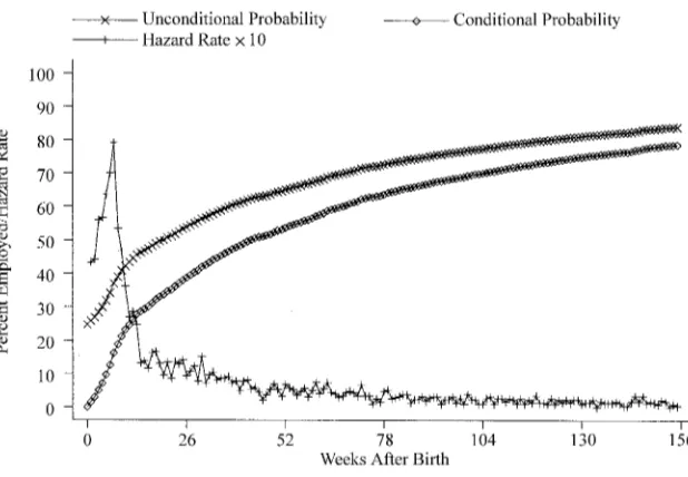
Figure 1
Employment Probabilities and Hazard Rates of Pregnant Women in Weeks Be-fore Birth
Figure 2
so until giving birth. The “conditional” estimates show employment probabilities for those with some pregnancy work experience and demonstrate that one-third of such women remain employed until delivery. Weekly hazard rates out of employment (dis-played in percentages multiplied by 5) are less than 2 percent per week during the rst two trimesters, increase to around 3 percent in the seventh month, 4 to 5 percent in month eight, and then rise to almost 20 percent in the week before delivery.
Figure 2 summarizes reemployment rates following birth. One-fourth of mothers are absent from jobs less than one week after delivery, although some “employed” women may initially be on maternity leave. Weekly reemployment hazard rates aver-age 4 to 8 percent for the next 10 weeks, decline rapidly to 1 to 2 percent in the fourth through sixth months of the child’s life, and are less than 1 percent for the remainder of the rst year. The hazard rates typically range between 0.2 and 0.6 percent per week during the second year and 0.1 to 0.2 percent in Year 3. Sixty-ve, 77, and 84 percent of women return to jobs prior to their child’s rst, second, and third birthday, as do 53, 70, and 79 percent of those taking some time off work after birth.
B. Paternal Employment
Most mothers remain home with infants for a substantial period of time. Fathers do not. Sixty-four percent work in every week of Year 1, 84 percent in at least four-fths of the weeks, only 3 percent do not hold a job at any point of the year, and just 8 percent work less than 26 weeks.37Similarly, 41 percent of fathers are em-ployed every week of the rst three years, 84 percent in at least 80 percent of weeks, less than 1 percent never hold a job, and fewer than 4 percent work less than half the weeks.
There are four reasons to believe that most weeks away from jobs donotoccur because fathers are choosing to spend time with young children. First, nonemploy-ment is evenly distributed across the rst three years, rather than being concentrated in the Year 1, as expected if the absences are motivated by a desire to be with infants.38Second, more than half (53 percent) of nonemployment is spent on tempo-rary layoff or looking for a job, suggesting that most work absences are involuntary.39 Third, fathers with substantial joblessness possess characteristics associated with employment instability, so that their nonemployment may be due to these factors.40 Fourth, time-diary evidence presented by Hofferth (2001) indicates that nonworking fathers spendlesstime with their children than employed men.
As with women, there is substantial bunching of paternal employment in weeks of work around 40 hours —55 to 59 percent work exactly this amount in each of
37. Information in this section refers to fathers living with children in the nationally representative subsam-ple of the NLSY at the survey date of the fourth year after birth.
38. Among fathers jobless less than six months during the three years (84 percent of the sample), 34, 35, and 31 percent of weeks of nonemployment take place during years one, two, and three. By contrast, 63 percent of the weeks corresponding mothers are off work occur during the rst year and just 22 percent in Year 3.
39. A larger proportion of nonemployment is devoted to job search or spent on layoff in Year 1 than in Years 2 and 3. This is not expected if fathers are choosing to invest time in infants.
Years 1 through 3. However, in sharp contrast to mothers, a large proportion of fathers supply considerably more labor. For instance, 38, 29, and 12 percent average 45, 50, and 60 or more hours of work per week in Year 1, versus 11, 6, and 2 percent of mothers.41
C. Descriptive Relationships
Early maternal employment is associated with relatively high levels of cognitive achievement. The rst three rows of Table 1 show that children whose mothers worked 30 or more hours per week during the early years scored a statistically sig-nicant 0.2 to 0.3 standard deviations higher on the PPVT, PIAT-R, and PIAT-M tests than those with nonworking mothers.
The remainder of the table demonstrates that these differences mostly donot re-ect a causal effect of the labor supply. Instead, children with employed mothers come from advantaged families and possess characteristics associated with advanced development. For instance, women working 30 or more hours per week during the child’s rst year are more educated and have higher AFQT scores than those not holding jobs. They are also less likely to be poor before pregnancy (6 versus 30 percent), unmarried at childbirth (30 versus 42 percent), and to have the father absent from the household in the fourth calendar year after birth (20 versus 29 percent). Similarly, the children of these mothers less often have low birthweight and require hospitalization before their rst birthday, both of which proxy poor health.
These ndings indicate the need for a careful multivariate investigation. If disad-vantaged family backgrounds or child health problems retard cognitive development and are associated with reduced labor supply, failing to correct for this heterogeneity will lead to upward biased estimates of the return to parental employment. The con-clusions of many previous analyses that include only rudimentary controls are there-fore likely to be overly optimistic.
VI. Regression Estimates
Table 2 summarizes the results of nine econometric specications for each of the three cognitive outcomes. The dependent variables in Models a through f and i are standard test scores, normalized to have a standard deviation of one. Col-umns g and h show ndings for similarly normalized percentile and raw scores. Maternal employment refers to average weekly work hours (divided by 20) in the specied period, except for Model h which examines the fraction of weeks worked (multiplied by two).42Year 0 includes the four quarters prior to birth; Years 1, 2, and 3 to the rst through fourth, fth through eight, and ninth through twelfth quar-ters after it. All models include assessment year dummy variables. Additional re-gressors are detailed at the bottom of the table:B,S,A, andErefer to the vectors
41. The corresponding gures are 40, 29, and 13 (12, 7, and 2) percent for fathers (mothers) in Year 2 and 42, 31, and 14 (14, 8, and 2) percent in Year 3.
T
h
e
Journal
of
H
um
an
R
es
ourc
es
Table 1
Sample Means of Selected Variables By Weekly Work Hours of the Mother
Average Weekly Work Hours Average Weekly Work Hours During Year 1 During Years 2 and 3 Full
Variable Sample 0 1–29 $30 0 1–29 $30
Cognitive outcomes
PPVT 0.00 20.15 0.09 0.10 20.21 0.08 0.07
(0.02) (0.04) (0.03) (0.04) (0.05) (0.03) (0.03)
PIAT-R 0.00 20.10 0.04 0.11 20.17 0.03 0.10
(0.02) (0.03) (0.03) (0.04) (0.04) (0.03) (0.04)
PIAT-M 0.00 20.11 0.05 0.11 20.16 0.04 0.08
(0.02) (0.03) (0.03) (0.04) (0.04) (0.03) (0.03) Family Background Characteristics
Mother’s age at birth (years) 24.7 24.3 24.4 25.9 24.8 24.1 25.6 (0.1) (0.1) (0.1) (0.1) (0.1) (0.1) (0.1) Mother’s education (years) 12.5 12.0 12.7 13.2 12.0 12.4 13.1
(0.0) (0.1) (0.1) (0.1) (0.1) (0.1) (0.1) Mother’s AFQT score 67.9 61.9 70.6 73.8 61.5 68.4 72.6
R
uhm
171
Mother’s work hours in fourth quar- 21.7 11.3 23.4 37.4 10.7 20.3 33.7 ter before birth (0.3) (0.5) (0.5) (0.5) (0.6) (0.5) (0.5) Father in household in fourth calen- 75.8 71.2 77.9 80.3 72.5 76.9 76.5 dar year after birth (%) (0.8) (1.3) (1.2) (1.5) (1.6) (1.1) (1.4) Family in poverty in 2ndyear before 18.8 29.9 14.4 6.3 31.2 18.5 8.4
birth (%) (0.7) (1.4) (1.1) (0.9) (1.7) (1.1) (0.1) Child Characteristics
Low birth weight (%) 6.5 7.7 5.8 5.5 8.6 5.4 6.2
(0.4) (0.8) (0.7) (0.9) (1.0) (0.6) (0.8) Preterm birth (%) 19.7 19.6 19.2 20.9 21.0 18.0 21.1
(0.7) (1.1) (1.2) (1.5) (1.4) (1.0) (1.4) Hospitalized during rst year of life 7.4 8.4 7.3 5.7 7.8 8.2 5.9
(%) (0.5) (0.8) (0.8) (0.9) (0.9) (0.7) (0.8)
T
h
e
Journal
of
H
um
an
R
es
ourc
es
Table 2
Regression Estimates of the Effects of Maternal Employment on Child Cognitive Development
Time Period (a) (b) (c) (d) (e) (f) (g) (h) (i)
Dependent Variable: PPVT Score
Year 1 0.054 20.039 20.045 20.073 20.065 20.073 20.103 20.076 20.061 (0.029) (0.024) (0.024) (0.027) (0.027) (0.027) (0.027) (0.024) (0.026) Years 2 and 3 0.097 0.056 0.016 0.024 0.030 0.022 0.017 0.016 0.024
(0.027) (0.023) (0.023) (0.028) (0.028) (0.028) (0.028) (0.025) (0.028)
Year 0 0.043 0.050 0.039 0.078 0.061 0.041
(0.028) (0.028) (0.028) (0.028) (0.025) (0.031) Dependent Variable: PIAT-R Score
Year 1 0.091 0.021 0.011 20.030 20.028 20.032 20.031 20.028 20.058 (0.027) (0.025) (0.025) (0.029) (0.029) (0.029) (0.029) (0.025) (0.028) Years 2 and 3 0.055 20.010 20.043 20.080 20.081 20.079 20.074 20.067 20.056
(0.026) (0.024) (0.024) (0.029) (0.029) (0.029) (0.029) (0.026) (0.029)
Year 0 0.030 0.030 0.029 0.033 0.016 0.072
R
uhm
173
(0.027) (0.025) (0.025) (0.029) (0.029) (0.029) (0.029) (0.026) (0.028) Years 2 and 3 0.041 23.2E-4 20.031 20.057 20.059 20.057 20.060 20.045 20.060
(0.026) (0.024) (0.024) (0.030) (0.030) (0.030) (0.030) (0.026) (0.030)
Year 0 0.033 0.037 0.031 0.041 0.016 0.061
(0.030) (0.030) (0.030) (0.030) (0.026) (0.033)
Additional regressors None B B,S B,S,E B,S,E,A B,S,E,I B,S,E B,S,E B,S,E Dependent variable Standard Standard Standard Standard Standard Standard Percen- Raw Standard
Score Score Score Score Score Score tile Score Score Score
Employment variable Hours Hours Hours Hours Hours Hours Hours Hours Weeks
of basic, supplemental, auxiliary, and maternal employment characteristics described previously and detailed in the appendix (Table A1);Iindicates total family income ($1996) during the calendar year before birth and the next four years.43
One empirical strategy is to examine how the addition of more complete controls alters the parameter estimates on maternal labor supply. A second is to pay special attention to the coefcient on work hours in the year prior to birth. As discussed, a small and insignicant parameter suggests that the other covariates adequately ac-count for nonrandom selection into employment based on maternal or family (but possibly not child) characteristics, whereas a large or statistically signicant coef-cient may indicate remaining omitted variables bias.
A. Verbal Skills of Three- and Four-year-olds
The top three rows of Table 2 display results for PPVT scores. As in the descriptive analysis, three- and four-year-olds with employed mothers have relatively high ver-bal ability. In Column a, which controls only for work hours and the assessment year, 20 hours of employment per week during the child’s rst (second and third) year is associated with a 0.05 (0.10) standard deviation rise in verbal performance. However, this positive relationship largely results from omitted variables bias, rather than from any causal effect of maternal job-holding. Thus, the inclusion of the basic set of covariates (Specication b) cuts the parameter estimate for Years 2 and 3 by more than 40 percent and switches the Year 1 coefcient from positive to negative. These results closely resemble those of much previous research using similar models in suggesting harmful “effects” of maternal employment during the rst year but with roughly offsetting benets for working during the next two.
Adding controls for supplemental and maternal employment characteristics yields more negative results (Columns c and d). For instance, in Specication d, 20 extra employment hours weekly throughout the rst three years is correlated with a 0.05 standard deviation decline in PPVT scores. The year zero coefcient is substantial (0.043) in this model and estimated fairly precisely, however, suggesting that even the extensive set of explanatory variables may not adequately account for heteroge-neity. This issue receives further attention below. Holding the auxiliary characteris-tics constant has little effect on the parameter estimates (Model e) and so, except where noted, they are excluded from the remainder of the analysis.
Maternal employment could benet children by raising earnings. However, as shown in Column f, controlling for family incomes does not change the hours coef-cients. One explanation is that work may be associated with decreases in other sources of nancial support (such as transfer payments or spousal earnings) for some families, so that incomes do not rise much. Another is that the direct income effect, estimated from the regressions, is extremely small.44
The negative predicted impact of job-holding in Year 1 is somewhat greater when considering percentile rather than standard scores (Specication g) and that for
ployment in Years 2 and 3 is slightly smaller for the raw scores (Column h), but neither difference is large or signicant and the coefcient on prebirth work hours suggests that heterogeneity may be less well controlled for in these models. Holding weeks rather than hours of work constant (Model i) attenuates the estimated effect of working in the rst year (which is not surprising since some hours variation occurs during weeks of employment) but only slightly. Thus, the estimated impact of mater-nal employment is relatively robust to these changes and Model d is the specication focused upon in the remainder of the analysis.
B. Are the Results Consistent Across Alternative Cognitive Assessments?
PIAT-R and PIAT-M scores are the dependent variables in the fourth through ninth rows of Table 2. As with the PPVT test, more complete controls yield less favorable estimated impacts of maternal labor supply. Absent covariates other than the survey year, there is a positive association between work and child achievement (Column a). This correlation shrinks and loses statistical signicance or becomes negative when the “basic” regressors are included (Model b), declines further with the addition of the supplemental variables (Specication c), and decreases still more when mater-nal employment characteristics and prebirth work hours are held constant (Column d). The results are essentially unaffected by the addition of the auxiliary covariates or family incomes (Specications e and f), and broadly similar estimates are obtained when percentile or raw scores are the dependent variables (Models g through h), or when weeks rather than hours of work are controlled for (Column i).
These similarities notwithstanding, early employment is predicted to have a mark-edly more negative impact on PIAT-R and PIAT-M achievement than PPVT scores. Most striking is the strong estimated negative effect for working during Years 2 and 3, in contrast with the small positive correlation for PPVT performance. For instance, in Specication d, 20 hours of additional employment per week during the second and third years is associated with statistically signicant 0.08 and 0.06 standard deviation reduction in the reading and mathematics assessments. Twenty extra hours per week throughout the rst three years is correlated with 0.11 and 0.08 standard deviation decreases in these scores, versus a smaller 0.05 standard deviation decrease in PPVT performance. These correspond to drops in test scores from the median to the 46th, 47th, and 48thpercentiles respectively.
C. Remaining Heterogeneity
purging the estimated effects of employment during the child’s rst three years of remaining heterogeneity.46Therefore, I adopt the limited strategy of using the pre-birth parameter to test for omitted variables bias but do not further correct for the latter. As mentioned, the year zero coefcients are relatively large and close to sig-nicance for PPVT scores. By contrast, their smaller magnitude suggests that uncon-trolled heterogeneity is less of an issue for the PIAT-R or PIAT-M assessments.
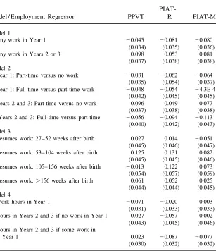
D. Intensity, Timing and Interaction Effects of Early Maternal Employment
Some previous researchers (for example, Waldfogel, Han and Brooks-Gunn, 2002) focus on the distinction between any versus no employment, rather than on the num-ber of work hours. For comparison, the rst model in Table 3 provides results with average work hours are replaced by dummy variables indicating whether the mother was employed during the specied period. These models distinguish working from not working but do not examine differences in intensity among mothers holding jobs. The results suggest benets of specializing in home production during the child’s rst year and of engaging in at least some market labor during the next two.
Model 2 allows for nonlinearities by separating part-time and full-time jobs, using 30 hours per week as the threshold between the two.47The estimates imply that part-time employment yields larger benets or lower costs than full-part-time work. Working part-time in the rst year is associated with 0.03, 0.06, and 0.06 standard deviation reductions in PPVT, PIAT-R, and PIAT-M scores compared to no employment; the PPVT and PIAT-R assessments are estimated to be anadditional 0.05 standard deviations lower when women hold full-time jobs, with no difference for the PIAT-M test. The disparities are even sharper in Years 2 and 3, where part-time work is correlated with substantial increases in all three cognitive measures (by 0.10, 0.05, and 0.08 standard deviations) but the expected scores are 0.06, 0.09, and 0.11 stan-dard deviations lower for full-time than part-time employment.
The third model shows results for dummy variables indicating the timing of the return to employment.48The ndings suggest that cognitive development is enhanced by nonmarket activities during the child’s rst year and that investments extending into the second and third year may also improve performance. Compared to starting work within six months, staying at home through at least a portion of the second year is correlated with 0.13, 0.13, and 0.08 standard deviation increases in PPVT, PIAT-R and PIAT-M scores. The anticipated gains in math and reading achievement are almost as large for children whose mothers are out of the labor market for two to three years, although still longer absences yield smaller expected benets.49 birth (prior to pregnancy) was generally positive and large in specications with limited controls but de-clined in size as heterogeneity was more completely accounted for.
46. Using the notation of Equation 12, the additional covariates sometimesincreasedbˆ by approximately
the same amount thatdˆ declined. In other casesbˆ changed little or decreased by a similar amount. These
three scenarios alternatively suggest usingbˆ2dˆ,bˆ, orbˆ1dˆ to provide heterogeneity-corrected estimates
of the effect of maternal employment during the child’s early years. 47. Similar results are obtained using 25 or 35 hours per week as the cutoff. 48. Women returning to jobs within six months are the reference group.
Table 3
Alternative Regression Estimates of the Effects of Maternal Employment
PIAT-Model / Employment Regressor PPVT R PIAT-M
Model 1
Any work in Year 1 20.045 20.081 20.080
(0.034) (0.035) (0.036)
Any work in Years 2 or 3 0.098 0.053 0.081
(0.037) (0.038) (0.038) Model 2
Year 1: Part-time versus no work 20.031 20.062 20.064 (0.035) (0.054) (0.037) Year 1: Full-time versus part-time work 20.048 20.054 24.3E-4
(0.042) (0.045) (0.045) Years 2 and 3: Part-time versus no work 0.096 0.049 0.077
(0.037) (0.038) (0.038) Years 2 and 3: Full-time versus part-time 20.056 20.094 20.113
(0.040) (0.042) (0.043) Model 3
Resumes work: 27–52 weeks after birth 0.027 0.014 20.051 (0.045) (0.046) (0.047) Resumes work: 53–104 weeks after birth 0.125 0.131 0.082
(0.045) (0.045) (0.046) Resumes work: 105– 156 weeks after birth 20.013 0.122 0.073
(0.054) (0.057) (0.059) Resumes work:.156 weeks after birth 0.061 0.052 0.025
(0.044) (0.044) (0.045) Model 4
Work hours in Year 1 20.071 20.020 0.003
(0.031) (0.033) (0.033) Hours in Years 2 and 3 if no work in Year 1 0.027 20.057 0.002
(0.043) (0.045) (0.046) Hours in Years 2 and 3 if some work in
Year 1 0.023 20.087 20.077
(0.030) (0.032) (0.032)
In the last model, the impact of employment during Years 2 and 3 is allowed to differ depending on whether the mother worked in the rst year. The results suggest more favorable effects if no job was held during the child’s infancy: working 20 hours weekly in Years 2 and 3 is estimated to lower PIAT-R assessments by 0.06 standard deviations if the mother did not hold a job in the rst year, with no effect predicted for PIAT-M performance, versus declines of 0.09 and 0.08 standard devia-tions if the mother worked during the rst 12 months.
These ndings modify our understanding of the relationship between maternal employment and child cognitive development in two ways. First, the uniformly nega-tive predicted effects of labor supply during Year 1 emphasize the special importance of investments during the child’s rst year and cast doubt on the possibility that infants suffer losses when their mothers work but “catch up” if the employment continues for the next two years. Second, limited employment during the second and third years is associated with higher test scores but these benets are predicted to decline or become negative as hours increase. Such results are consistent with child cognitive development being maximized by having the mother stay at home during the rst year and work limited amounts during the next two.
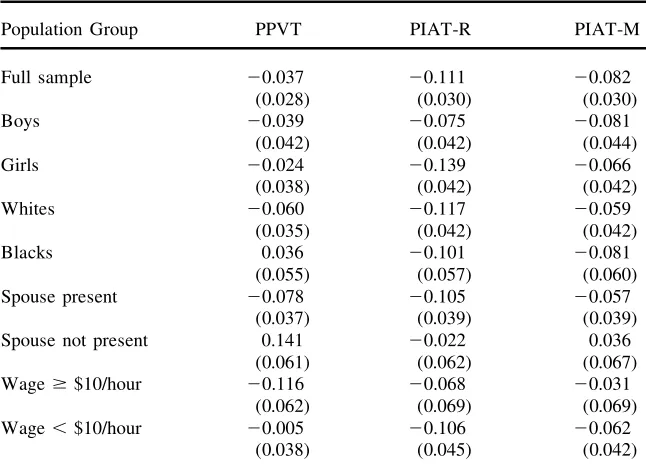
E. Subsamples
Table 4 provides results for population subgroups. The specications are identical to Model d of Table 2, except that work hours are averaged over all of the rst three years. Findings for the full sample, displayed in the rst row, conrm that maternal labor supply is modestly negatively correlated with PPVT scores but more strongly so with PIAT-R and PIAT-M performance—working 20 extra hours per week is estimated to reduce the three cognitive measures by 0.04, 0.11, and 0.08 stan-dard deviations, corresponding to declines from the median to the 49th, 46th, and 47th percentiles.
Some previous researchers (for instance, Desai, Chase-Lansdale and Michael 1989; Brooks-Gunn, Han and Waldfogel 2002) have found stronger negative effects for boys than girls; others (Han, Waldfogel and Brooks-Gunn 2000; Waldfogel, Han and Brooks-Gunn, 2002) suggest the deleterious impact is largely restricted to white children. The second through fth rows of the table test for, and largely reject, these possibilities. Maternal employment is estimated to lower the PPVT and PIAT-M scores of boys by more than girls but the reverse is true for the PIAT-R test.50 The negative relationship between work and PPVT or PIAT-R scores is stronger for whites than blacks but with the opposite pattern for the PIAT-M test.51
50. Han, Waldfogel, and Brooks-Gunn (2001) and Hill et al. (2001) similarly fail to uncover any gender differences in the impact of rst year employment; Waldfogel, Han, and Brooks-Gunn (2002) nd larger negative effects of full-time work for girls than boys.
Table 4
Estimates of the Effect of Maternal Employment on Alternative Groups of Children
Population Group PPVT PIAT-R PIAT-M
Full sample 20.037 20.111 20.082
(0.028) (0.030) (0.030)
Boys 20.039 20.075 20.081
(0.042) (0.042) (0.044)
Girls 20.024 20.139 20.066
(0.038) (0.042) (0.042)
Whites 20.060 20.117 20.059
(0.035) (0.042) (0.042)
Blacks 0.036 20.101 20.081
(0.055) (0.057) (0.060)
Spouse present 20.078 20.105 20.057
(0.037) (0.039) (0.039)
Spouse not present 0.141 20.022 0.036
(0.061) (0.062) (0.067)
Wage $$10/hour 20.116 20.068 20.031
(0.062) (0.069) (0.069)
Wage ,$10/hour 20.005 20.106 20.062
(0.038) (0.045) (0.042)
Note: See note on Table 2. This table shows coefcients on average weekly work hours measured through-out the rst three years of the child’s life. These are obtained from models controlling for the same variables as Specication d of Table 2. The second and third rows divide the sample between boys and girls. The fourth and fth provide separate estimates for non-Hispanic whites and non-Hispanic blacks (with Hispan-ics excluded). The sample in the sixth row is restricted to children whose mothers have a spouse in the household at each of the survey dates in the rst three calendar years following birth; that in the seventh refers to children whose mothers do not have a spouse living in the household at any of the three survey dates. The eighth and ninth rows stratify the sample by the hourly wage (in $1996) of the mother in the fourth quarter prior to the child’s birth; women not working at that time are excluded. The number of observations ranges from 4,180 to 4,803 for the full sample, 2,099 to 2,443 for boys, 2,081 to 2,360 for girls, 2,159 to 2,327 for whites, 1,204 to 1,481 for blacks, 2,479 to 2,727 for children in households with a spouse present, 1,067 to 1,270 for those in household without a spouse present, 786 to 805 for children whose mothers earned at least $10/hour, and 1,770 to 2,031 for those whose mothers earned less than $10/hour.
The sample in the sixth and seventh rows is divided by whether a spouse (not necessarily the biological father) is in the household duringallornoneof the survey dates in the three calendar years following the child’s birth.52Given the relatively small sample sizes, the employment coefcients are estimated imprecisely. Never-theless, the results hint that maternal job-holding may be more harmful for two-parent than female-headed households. Hill et al. (2001) and Brooks-Gunn, Han and Waldfogel (2002) similarly nd more negative effects for children of married than
unmarried women. Possible explanations are that the home environment or parental time investments are of relatively high quality in two-adult families or that the earn-ings of mothers are especially benecial in female-headed households.53
The last two rows divide the sample into children of employed women earning more or less than $10 per hour ($1996) in the quarter before pregnancy.54Maternal labor supply is negatively related to the PPVT scores of children of high but not low earners, as expected if the mother’s earnings yield relatively large benets when wages are low. However, a similar result is not obtained for the R or PIAT-M assessments.
F. Childcare
Child care has been ignored until now out of concern that its use is inuenced by work decisions, so that controlling for it inappropriately attenuates the effects of maternal employment.55However, the impact of market labor could also vary with day care arrangements. For instance, deleterious consequences of employment dur-ing the child’s early years might reect the low average quality of nonparental care in the United States.56Some information on this issue was obtained by estimating models that added interactions between employment hours and the use or mode of day care.57The restricted nature of this analysis is dictated by the limited child care data in the NLSY—there is information on the number and type of arrangements but not (after 1989) on the intensity, cost, or quality of care.
The regression estimates (not shown) fail to uncover any consistent effect of day care. Child care during the rst year is associated with slightly lower predicted verbal ability at ages three or four but marginally higher mathematics achievement two years later (with no difference in reading). Conversely, care in Years 2 and 3 is linked with higher (lower) PPVT and PIAT-M (PIAT-R) scores, and none of these correlations are close to being statistically signicant. The data also hint that center-based care during the second and third years may yield some benets but again the estimates are imprecise. Generally, these results conform to prior research ndings of small and inconsistent effects of nonparental care. Most importantly, the coef-cients on maternal employment do not change much with the inclusion of controls for day care.
53. However, the coefcients on prebirth work hours are fairly large for the nontraditional families (be-tween 0.04 and 0.06), raising the possibility of remaining heterogeneity.
54. Women not working at this time are excluded. Other wage thresholds were also considered. 55. Over 85 percent of NLSY mothers with children younger than the age of three and working at least 30 hours per week use nonparental care, compared to less than one-fth of nonemployed mothers. Day care rises with child age, from 44 percent in Year 1 to 54 percent in Year 3, because nonworking mothers more often place toddlers (than infants) in care and women with older children are increasingly likely to work. The rise between the rst and third year is entirely accounted for by growth in center-based care. 56. Helburn and Howes (1996) indicate that 86 percent of day care centers provide “mediocre or poor” services and that only 9 percent of family child care homes supply “good” quality care.
57. The modes include relative, center-based, and other types of nonparental care. The regression model is:Cit5a1Xitb1Hit2jg1Hit2jDit2jd1eit, whereDit2jindicates either whether nonparental care is
G. Alternative Specications
To ensure that the disparate ndings obtained for PPVT and PIAT scores do not reect differences in the samples (primarily occurring due to the varying ages at which the tests are given), I estimated models for the 3,045 children with scores reported for all three cognitive assessments. The results conrm that employment is more strongly negatively related to PIAT-R and PIAT-M achievement than PPVT performance: 20 extra hours per week throughout the rst three years is associated with20.08,20.11, and20.03 standard deviation reductions in three test scores for this group (with standard errors of 0.03, 0.04, and 0.03).
The effects were allowed to differ across high and low achievers through a series of quantile regression models examining the 10th, 25th, 50th, 75th, and 90thpercentiles of test performance. These estimates failed to reveal any disparate impact across achievement levels for the PIAT-R and PIAT-M assessments. However, employment was predicted to have more negative impacts on high than low PPVT scores: the coefcient (standard error) on average weekly hours in Years 1 through 3 was 0.03 (0.06), 20.01 (0.03),20.05 (0.03),20.06 (0.02), and20.06 (0.04) at the 10th, 25th, 50th, 75th, and 90thpercentiles.58
Fixed-effect models were estimated by restricting the sample to siblings and in-cluding a vector of mother-specic dummy variables. As discussed, these understate the costs of maternal employment if women supply less labor when their children have health or developmental problems. The results are consistent with this expecta-tion. Specically, the FE coefcients (standard errors) on PPVT, R and PIAT-M scores for labor supply throughout the rst three years are 0.04 (0.05), 20.08 (0.05) and20.07 (0.05); the corresponding OLS estimates are20.04 (0.03),20.13 (0.04), and 20.09 (0.04).59Thus, even with a likely upward bias, the xed-effect models suggest a negative relationship between early maternal employment and the reading or mathematics achievement of ve- and six-year-olds.
A nal set of specications controlled for the incidence or duration of breast-feeding, which has been linked to improved cognitive development (Anderson, John-stone, and Remley 1999). Working mothers are less likely to breast-feed, which could explain a portion of the negative effect of maternal employment (particularly during the rst year). However, the results provide little support for this. Breast-feeding is positively associated with the assessment scores but its inclusion only slightly attenuates the Year 1 labor supply coefcients and does not affect the param-eter estimates for work in Years 2 and 3.
VII. What about Fathers?
The preceding analysis suggests the importance of maternal invest-ments in young children. But what about fathers? While it is possible that mothers provide unique inputs, it seems likely that there is at least some substitutability be-tween parents. However, since men are typically paid more than women, larger in-come benets could accrue to paternal employment. These issues are addressed in