A PARAMETERIZED LOWER BOUND FOR THE SMALLEST
SINGULAR VALUE∗
WEI ZHANG†, ZHENG-ZHI HAN†, AND SHU-QIAN SHEN‡
Abstract. This paper presents a parameterized lower bound for the smallest singular value of
a matrix based on a new Gerˇsgorin-type inclusion region that has been established recently by these authors. The comparison of the new lower bound with known ones is supplemented with a numerical example.
Key words. Eigenvalue, Inclusion region, Smallest singular value, Lower bound.
AMS subject classifications.15A12, 65F15.
1. Introduction. To estimate matrix singular values is an attractive topic in matrix theory and numerical analysis, especially to give a lower bound for the smallest one. Let A = (aij) ∈Cn×n and letA∗ be the conjugate transpose of A. Then the singular values of A are the square roots of the eigenvalues of AA∗. Throughout the paper we use σn(A) to denote the smallest singular value of A. D enote N :=
{1,2, . . . , n}. Define, for allk∈N,
rk(A) :=
j∈N\{k}
|akj|, ck(A) :=
j∈N\{k}
|ajk|, hk(A) := 1
2(rk(A) +ck(A)).
In the past three decades, several useful lower bounds for the smallest singular value of a matrix have been presented in the literature; see Varah [7] and Qi [6]. By using Gerˇsgorin’s theorem (see Chapter 6 of [1]), Johnson [4] obtained a lower bound forσn(A):
(1.1) σn(A)≥min
k∈N{|akk| −hk(A)}.
Recently, Johnson and Szulc [5] provided several further lower bounds for the
∗Received by the editors August 14, 2008. Accepted for publication September 26, 2008. Handling
Editor: Roger A. Horn.
†School of Electronic, Information and Electrical Engineering, Shanghai Jiao Tong University,
Shanghai, 200240, China ([email protected]).
‡School of Applied Mathematics, University of Electronic Science and Technology of China,
Chengdu, 610054, China.
smallest singular value. Two of them are
(1.2) σn(A)≥ 1 2mink∈N
4|akk|2+ [rk(A)−ck(A)]2 12
−2hk(A)
and
(1.3) σn(A)≥ 1 2mini=k
|aii|+|akk| −
(|aii| − |akk|)
2
+ 4hi(A)hk(A) 12
.
In this paper, after introducing a new inclusion region for eigenvalues of a matrix in Section 2, we present a parameterized lower bound for the smallest singular value in Section 3. In Section 4, a numerical example is given to compare our results with the known ones.
2. Inclusion regions for eigenvalues. Recently, a new Gerˇsgorin-type inclu-sion region for eigenvalues of a matrix has been provided by Huang, Zhang, and Shen in [3]. To introduce the result, we first present some notation. LetS be a nonempty subset of N. D enote ¯S := N\S and let P(N) denote the power set of N. For
A= (aij)∈Cn×n, define, for alli∈N
rSi(A) :=
k∈S\{i}
|aik|, r
¯
S i(A) :=
k∈S¯\{i}
|aik|,
cSi(A) :=
k∈S\{i}
|aki|, c
¯
S i(A) :=
k∈S¯\{i}
|aki|.
If S contains a single element, say S = {i0}, then we let rS
i0(A) = 0. Similarly
rS¯
i0(A) = 0 if ¯S ={i0}. We sometimes use r
S i (cSi, r
¯
S i, c
¯
S
i) to denoterSi(A) (cSi(A),
rS¯ i(A),c
¯
S
i(A), respectively). Define, for alli∈S and j∈S¯,
GSi(A) :=
z∈C:|z−aii| ≤rSi , GSj¯(A) :=z∈C:|z−ajj| ≤rSj¯
and
GS i,j(A) :=
z∈C:z /∈GSi(A)∪GSj¯(A),
|z−aii| −rSi
|z−ajj| −r
¯
S j
≤rS¯ ir
S j
.
Proposition 2.1. ([3]) Let A = (aij) ∈ Cn×n. Then all the eigenvalues of A
are located in
GS(A) :=
i∈S
GSi(A)
∪
j∈S¯ GSj¯(A)
∪
i∈S,j∈S¯
GSi,j(A)
This result is interesting, but it can not be applied directly to estimate σn(A). So we must deduce other inclusion regions. Letα∈ [0,1] be given. For i ∈S, j ∈ S¯, define the following regions in the complex plane:
Ui,jS (A) :=
z∈C:|z−aii| −riS ≤riS¯rjS α
,
VS i,j(A) :=
z∈C:|z−ajj| −rjS¯≤riS¯rjS
1−α
,
Proposition 2.2. Let A = (aij) ∈ Cn×n. Then all the eigenvalues of A are
located in
KS(A) :=
i∈S,j∈S¯
US i,j(A)
∪
i∈S,j∈S¯
VS i,j(A)
.
Proof. It is sufficient to show thatGS(A)⊂KS(A). Note thatGS
i(A)⊆Ui,jS(A) andGS¯
j(A)⊆Vi,jS(A). Therefore, for anyz∈GS(A), if
z∈
i∈S
GSi(A) or z∈
j∈S¯
GSj¯(A),
thenz∈KS(A). Otherwise, there existi0∈S andj0∈S¯, such that
|z−ai0i0| −r
S i0
|z−aj0j0| −r
¯
S j0
≤rS¯ i0r
S j0 =
rS¯ i0r
S j0
α
rS¯ i0r
S j0
1−α
which leads to
|z−ai0i0| −r
S i0≤
rS¯ i0r
S j0
α
or |z−aj0j0| −r
¯
S j0 ≤
rS¯ i0r
S j0
1−α
.
Hence
z∈US
i0,j0(A)∪V
S i0,j0(A).
And thenz∈KS(A).
3. Main results. In this section we use the inclusions derived in Section 2 to estimateσn(A). Denote the Hermitian part of Aby
H(A) := 1 2(A+A
Letλmin(H(A)) be the smallest eigenvalue ofH(A). It is known thatλmin(H(A)) is a lower bound forσn(A) [2, p.227]. Moreover, define for alli∈S,j∈S¯, andα∈[0,1],
PS
i,j(A) : =|aii| −21riS(A) +c S i(A)
−1 4
rS¯ i(A) +c
¯
S i(A)
rS j(A) +c
S j(A)
α
,
QSi,j(A) : =|ajj| −12
rSj¯(A) +c
¯
S j(A)
−14riS¯(A) +c
¯
S i(A)
rjS(A) +c S j(A)
1−α
.
Theorem 3.1. Let A= (aij)∈Cn×n. Then
(3.1) σn(A)≥ min
i∈S,j∈S¯
PS i,j(A), Q
S i,j(A) .
Proof. We first define a diagonal matrixD=diag(eiθ1, . . . , eiθn),whereeiθka kk=
|akk|ifakk= 0 andθk = 0 ifakk= 0,k∈N. SinceD is unitary, the singular values ofDAare the same as those ofA. Consequently, we have
(3.2) σn(A) =σn(DA)≥λmin(H(DA)).
DenoteB = (bkl) :=H(DA) = 12(DA+A∗D∗).Thus,bkk=|akk|, fork∈N, and
bkl= 1 2
ekθk
akl+ ¯alke−kθk
, for all k=l, k, l∈N.
Since B is a Hermitian matrix, its eigenvalues are all real. Letλmin(B) denote the smallest eigenvalue ofB. Then, by using Proposition 2.2, λmin(B) must satisfy at least one of the following conditions
λmin(B)≥ |bii| −riS(B)−
rS¯ i(B)r
S j(B)
α
, i∈S, j∈S,¯
λmin(B)≥ |bjj| −r
¯
S j(B)−
riS¯(B)r S j(B)
1−α
, i∈S, j∈S.¯
It follows that
λmin(B)≥ min i∈S,j∈S¯
|bii| −rSi(B)−
rSi¯(B)r S j(B)
α
,
|bjj| −r
¯
S j(B)−
rS¯ i(B)r
S j(B)
1−α
.
By applying the triangle inequality, we have
|bii| −rSi(B)−
rSi¯(B)r S j(B)
α
=|aii| −riS(H(DA))−
rS¯
i (H(DA))r S
j (H(DA)) α
≥ |aii| −12
rS
i(A) +cSi(A)
−14rS¯ i(A) +c
¯
S i(A)
rS
j(A) +cSj(A) α
Similarly, one can obtain
|bii| −r
¯
S i (B)−
rS¯
i(B)rSj(B) 1−α
≥QS i,j(A).
Then from (3.2), we have
σn(A)≥ min i∈S,j∈S¯
PS
i,j(A), QSi,j(A) .
Since the bound (3.1) holds for any nonempty S ∈ P(N) and anyα∈[0,1], we have obtain the following corollaries:
Corollary 3.2. σn(A)≥ max
S∈P(N)αmax∈[0,1]i∈minS,j∈S¯
PS
i,j(A), QSi,j(A) .
Corollary 3.3. ([4]) σn(A)≥min
i∈N
|aii| −12(ri(A) +ci(A)) .
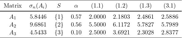
4. Numerical example. In this section, we give a numerical example to com-pare our bound (3.1) with known ones.
Example 4.1. Consider the following matrices
A1=
11 5 6
4 12 −5
3 4 13
, A2=
18 2 −5
6 15 8
−6 −3 17
, A3=
6 2 −1
2 9 1
2 −2 −13
.
Table 1. Comparison of lower bounds forσn(A)
Matrix σn(Ai) S α (1.1) (1.2) (1.3) (3.1)
A1 5.8446 {1} 0.57 2.0000 2.1803 2.4861 2.5886
A2 9.6861 {2} 0.56 5.5000 6.1172 5.7827 5.7989
A3 4.5433 {3} 0.10 2.5000 3.6921 2.3028 2.8377
[image:5.612.107.406.438.501.2]REFERENCES
[1] R. A. Horn and C. R. Johnson. Matrix Analysis. Cambridge University Press, Cambridge, 1985. [2] R. A. Horn and C. R. Johnson. Topics in Matrix Analysis. Cambridge University Press,
Cam-bridge, 1991.
[3] T. Z. Huang, W. Zhang, and S. Q. Shen. Regions containing eigenvalues of a matrix. Electron. J. Linear Algebra, 15:215–224, 2006.
[4] C. R. Johnson. A Gersgorin-type lower bound for the smallest singular value. Linear Algebra Appl., 112:1–7, 1989.
[5] C. R. Johnson and T. Szulc. Further lower bounds of the smallest singular value.Linear Algebra Appl., 272:69–179, 1998.
[6] L. Qi. Some simple estimates for singular values of a matrix. Linear Algebra Appl., 56:105–119, 1984.