Mathematics and Informatics ICTAMI 2005 - Alba Iulia, Romania
BIFURCATION IN A MODEL OF THE POPULATION DYNAMICS
Raluca-Mihaela Georgescu
Abstract. The static bifurcation diagram (sbd) and the global dynamic bifurcation diagram (dbd) around some nonhyperbolic equilibria are provided for the Odell model which depends on one parameter. The biological interpre-tation is then presented.
2000 Mathematics Subject Classification: 37N25, 34C23.
1. The mathematical model
Predator-prey models govern many phenomena in population dynamics, immunology, medicine etc. We assume that there are only two competing species: one species (predator) feeds on another species (prey), which in turn feeds on other things. We deal with a particular case of the model consisting of a Cauchy problem x(0) =x0, y(0) =y0, for the following system of ordinary differential equations (sode), which was studied by Odell in 1980 [6]
˙
x = x[x(1−x)−y], ˙
y = y(x−a), (1)
wherexandy represent the population numbers of the prey and the predator, respectively, andais a nonnegative parameter. The presence of this parameter is the source of a rich dynamics generated by (1) and of its qualitative changes as a crosses some values on the real axis.
In this paper we study only the biologically realistic case a > 0 and we treat the bifurcation from a new perspective [3].
2.The static bifurcation diagram
If a /∈ {0,1} there exist three equilibrium points: O(0,0), E1(1,0), E2(a, a(1 −a)). If a = 1 the point E1 collides with E2 and, in this way, there are only two equilibrium points, O and E1.
We recall that the attractivity properties of an equilibrium point (x∗, y∗)
is determined by the real part of the eigenvalues of the matrix A defining the linearized sode about this point. In our case
A=
2x−3x2
−y −x
y x−a
. (2)
Therefore, O is a saddle-node (the eigenvalues of A are λ1 = 0, λ2 =−a) and E1 is a saddle for a <1, a saddle-node for a = 1 and an attractive node for a > 1 (the eigenvalues of A are λ1 = −1, λ2 = 1−a). For the third equilibrium point, E2, the eigenvalues of the matrix A are the roots of the characteristic equation
λ2
−tr A λ+ detA= 0, (3)
with tr A=a(1−2a), detA=a2
(1−a) and ∆ =a2
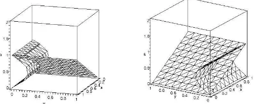
(4a−3). Therefore, the point E2 is a repulsive focus for a ∈ (0,1/2), a Hopf singularity for a = 1/2, an attractive focus for a ∈ (1/2,3/4), a sink for a = 3/4, an attractive node for a ∈ (3/4,1), a saddle-node for a = 1 and a saddle for a > 1. In this last case, the point E2 is in the fourth quadrant.
[image:2.612.170.421.485.588.2]As a consequence, as we said in the above, we can construct the sbd, represented in fig. 1 from two perspectives.
Owing to the Hartman-Grobman theorem, we are interested only in non-hyperbolic equilibria: the saddle-node O for a∈R+\ {0}, the saddle-nodeE1 for a= 1 and the Hopf singularity E2 for a = 1/2.
3.The nature of the nonhyperbolic equilibrium points
In order to see whether a nonhyperbolic equilibrium point is a degenerated or a nondegenerated singularity we have to derive the normal form of (1) at that point [1].
Proposition 1. The normal form of (1) at O(0,0) for a6= 0 is
˙
n1 = n2
1+O(n 3
), ˙
n2 = −an2+n1n2+O(n3
), (4)
and, thus, O is a nondegenerated saddle-node. The system (1) is equivalent to
˙
x = x2
−xy+O(x3 ), ˙
y = −ay+xy,
(5)
whose matrix of the linear terms is diagonal. In order to reduce the second order nonresonant terms in (5) we determine the transformationX=n+h(n), where X= (x, y)T and n= (n1, n2)T, suggested by the Table 1.
m1 m2 Xm,1 Xm,2 Λm,1 Λm,2 hm,1 hm,2
2 0 1 0 0 a - 0
1 1 -1 1 −a 0 1/a
-0 2 0 0 −2a −a 0 0
Table 1.
Here Λm,1, Λm,2 are the eigenvalues of the associated Lie operator, and Xm is a second order vector polynomial in (5). We find the transformation
x = n1+ (1/a)n1n2, y = n2,
Proposition 2. The normal form of (1) at E1(1,0)for a = 1 is
˙
n1 = −n1−4n1n2 +O(n3 ), ˙
n2 = n2
2+O(n 3
), (6)
and, thus, E1 is a nondegenerated saddle-node.
Proof. First, we translate the point E1 at the origin with the aid of the change u1 =x−1, u2 =y. Letu= (u1, u2)T. Then, in u, (1) reads
˙
u1 = −u1−u2−2u2
1−u1u2−u 3 1, ˙
u2 = u1u2. (7)
The eigenvalues of the matrix defining the linear terms in (7) are λ1 = −1, λ2 = 0 and the corresponding eigenvectors read uλ
1 = (1,0)
T
and uλ
2 = (1,−1)
T. Thus, with the change of the coordinates
u1 u2
=
1 1 0 −1
v1 v2
,(7) achieves the form
˙
v1 = −v1−2v2
1 −4v1v2−2v 2
2 +O(v 3
), ˙
v2 = v1v2 +v2
2, (8)
involving a diagonal matrix of the linear terms. In order to reduce the second order nonresonant terms in (8) we determine the transformationv=n+h(n), where v= (v1, v2)T and n= (n1, n2)T, suggested by the Table 2.
m1 m2 Xm,1 Xm,2 Λm,1 Λm,2 hm,1 hm,2
2 0 -2 0 -1 -2 2 0
1 1 -4 1 0 -1 - -1
0 2 -2 1 1 0 -2
-Table 2.
Here Λm,1, Λm,2 are the eigenvalues of the associated Lie operator and Xm is a second order vector polynomial in (8). We find the transformation
v1 = n1+ 2n2 1−2n
carrying (8) into (6). By [1], the equilibrium pointE1(1,0) corresponding the dynamical system generated by a sode of the form (6) is a nondegenerated saddle-node.
Proposition 3. The normal form of (1) at E2(1/2,1/4) for a= 1/2 is ˙ w1 ˙ w2 =
0 −√2/4
√
2/4 0
−(w2 1+w
2 2) " 1 2 w1 w2 +31 √ 2 18
−w2
w1 #
+O(w4
)
(9)
and, thus, E2 is a nondegenerated Hopf singularity.
Proof. First, we translate the point E2 at the origin with the aid of the change u1 =x−1/2, u2 =y−1/4. Letu= (u1, u2)T. Then, inu, (1) reads
˙
u1 = −1 2u2−
1 2u
2
1−u1u2 −u 3 1,
˙
u2 = 1
4u1+u1u2.
(10)
The eigenvalues of the matrix defining the linear terms in (10) are λ1 = λ2 = √2i/4 and, let uλ
1 = (i √
2,1)T be an eigenvector
correspond-ing to the positive eigenvalue. We have uλ
1 = (0,1)
T +i(√2,0)T.Thus, with
the change of the coordinates
u1 u2
=PMC
v1 v2
,whereP= √
2 0
0 1
andMC= 1 2
1 1 −i i
, i.e. u1 u2 = 1 2 √
2 √2 −i i
v1 v2
,(10) achieves the complex form
˙ v1 = √ 2i 4 v1+
√ 2 8 + i 4 ! v2 1 − √ 2 4 v1v2−
3√2
8 + i 4 ! v2 2 − 1
4(v1+v2) 3
,
˙
v2 = − √
2i 4 v2−
3√2
8 − i 4 ! v2 1− √ 2
4 v1v2+ √ 2 8 − i 4 ! v2 2 − 1
4(v1+v2) 3
,
m1 m2 Xm,1 Xm,2 Λm,1 Λm,2 hm,1 hm,2
2 0 M N √2i/4 3√2i/4 P Q
1 1 √2/4 −√2/4 −√2i/4 √2i/4 −i i
0 2 N M −3√2i/4 −√2i/4 Q P
Table 3.
Here Λm,1, Λm,2 are the eigenvalues of the associated Lie operator, Xm is a second order vector polynomial in (11) M =
√ 2 8 +
i
4, N = − 3√2
8 − i 4, P = √ 2 2 − i
2 and Q= √
2 6 −
i 2 . We find the transformation
v1 = n1+ √ 2 2 − i 2 ! n2
1−in1n2+ √ 2 6 − i 2 ! n2 2,
v2 = n2+ √ 2 6 + i 2 ! n2
1+in1n2+ √ 2 2 + i 2 ! n2 2,
carrying (11) into ˙ n1 = √ 2i 4 n1 +
1 6 − √ 2i 2 ! n3 1− 1 2+
31√2i 18 ! n2 1n2− − 1 6+
7√2i 6 ! n1n2 2− 5 6 + √ 2i 2 ! n3
2+O(n 4
),
˙
n2 = − √
2i 4 n2−
5 6 − √ 2i 2 ! n3 1− 1 6−
7√2i 6
! n2
1n2−
− 12− 31 √ 2i 18 ! n1n2 2+ 1 6+ √ 2i 2 ! n3
2+O(n 4
).
(12)
m1 m2 Xm,1 Xm,2 Λm,1 Λm,2 hm,1 hm,2
3 0 R Z √2i/2 √2i C E
2 1 S T 0 √2i/2 - D
1 2 T S −3√2i/2 0 D
-0 3 Z R −√2i −√2i/2 E C
Table 4.
Here Xm is a third order vector polynomial in (11) R = 1 6 −
√ 2i 2 , S = −1
2 −
31√2i
18 , T = − 1 6 −
7√2i
18 , Z = − 5 6 −
√ 2i
2 , C = −1− √
2i 6 , D= 7
3− √
2i
6 , and E = 1 2−
5√2i 12 . We find the transformation
n1 = s1− 1 + √ 2i 6 ! s3 1+ 7 3 − √ 2i 6 ! s1s2 2+ 1 2−
5√2i 12
! s3
2,
n2 = s2+ 1 2+
5√2i 12 ! s3 1+ 7 3 + √ 2i 6 ! s2
1s2− 1− √ 2i 6 ! s3 2,
carrying (12) into ˙ s1 = √ 2i 4 s1−
1 2 +
31√2i 18
! s2
1s2+O(s4 ),
˙
s2 = − √
2i 4 s2−
1 2 −
31√2i 18
! s1s2
2+O(s 4
).
(13)
Let us come back to the real state functions by denotings1 =w1+iw2, s2 = w1−iw2 [4]. In this way we obtain
˙
w1 = − √
2i
4 w2−(w 2 1+w
2 2)
1 2w1−
31√2i 18 w2
!
+O(w4 ),
˙ w2 =
√ 2i
4 w1−(w 2 1+w
2 2) 1
2w1−
31√2i 18 w2
!
+O(w4 ), (14) or, equivalently, ˙ w1 ˙ w2 =
0 −√2/4
√
2/4 0
−(w21+w 2 2) " 1 2 w1 w2 +31 √ 2 18
−w2
w1 #
This is the normal form of (10). By [1], the equilibrium point E2(1/2,1/4) corresponding the dynamical system generated by a sode of the form (9) is a nondegenerated supercritical Hopf singularity.
4.The global dynamic bifurcation diagram
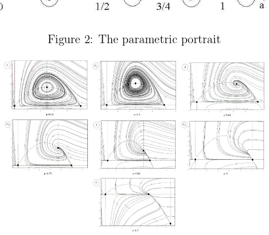
[image:8.612.160.431.329.566.2]The discussion in Section 2 shows on the reala−axis (which represents the parametric portrait) seven regions corresponding to topologically equivalent dynamical systems are determined (fig. 2). In fig. 3 we represent the phase portraits corresponding to each stratum of the parametric portrait. This shows that, in spite of their unrealistic significance for the population dynamics, the equilibria O, E1 and E2 for a > 1 heavily contribute to the changes in the phase portraits and, so, to the dynamic bifurcation diagram (which consists of figs 1 and 2).
Figure 2: The parametric portrait
Figure 3: Phase portrait for various strata in fig.2.
E1 is a saddle for any a < 1, a saddle-node for a = 1 and an attractive node for a >1; the equilibrium E2 is a repulsive focus, a Hopf singularity, an attractive focus, a sink, an attractive node, respectively, for different values of the parameter a <1. When a= 1, the equilibrium E2 collides withE1 and it becomes a saddle-node and, then, for a >1 it has a negative component, so, from the biological point of view, we can say that it disappears.
5.The biological interpretation
For mathematical reasons we studied the population dynamics for the entire real plane. However, for biology purposes we give the biological interpretation only for the fist quadrant. As a consequence, if x0 and/or y0 are negative we say that the corresponding equilibrium x0 = (x0, y0) does not exist.
Analyzing the portraits in fig. 3 we can conclude that, if one or both initial populations do not exist, they will not exist for ever and if the initial pop-ulations are at any equilibrium point, then the poppop-ulations remain constant at any subsequent time. For all other initial values the subsequent popula-tions vary in various manners, depending the values of the parameter a. The paths described by these values are phase space trajectories corresponding to transient regimes between some equilibrium state or/and periodic regime.
Thus, for the zones C1 and 2 the numbers of the subsequent populations are oscillatory but not periodic ( firstly both populations increase, then onlyy increases andx decreases, then onlyx increases andy decreases with the am-plitudes smaller and smaller, and again both populations increase and so on) until they reach the equilibrium pointE2. In the zone 2 the increase (decrease) of the populations are faster than in zone C1 where the increase (decrease) of the population is very very slow. For zones C3 and 3 the subsequent popu-lations are very little oscillatory until they come to an equilibrium point E2. For the zone 1, the equilibrium points are repulsive and the populations go to a limit cycle where they become periodic.
Finally, we can conclude that the prey x(t) flourish in the absence of the predator. Theoretically, the predator can destroy all the prey so that the latter becomes extinct. However, if this happens the predator y(t) will also become extinct since, as we assume, it depends on the prey for its existence. In addition, our parametric portrait shows where all these phenomena occur.
[1] Arrowsmith, D.K., Place, C.M., Ordinary differential equations, Chap-man and Hall, London, 1982.
[2] Chow, S.-N., Li, C., Wang, D., Normal forms and bifurcation of planar fields, Cambridge University Press, 1994.
[3] Georgescu, A., Dynamic bifurcation diagrams for some models in eco-nomics and biology, Journal, Proc. Intern. Conf. on Theory and Applications of Mathematics and Informatics - ICTAMI 2004, Thessaloniki, Greece, Acta Universitatis Apulensis, Mathematics-Informatics, 156-163.
[4] Georgescu, A., Georgescu, R.M.,Normal forms for nondegenerated Hopf singularities and bifurcations, Proc. Conf. on Applied and Industrial Mathe-matics - CAIM 2003, Oradea, Romania, 104-112.
[5] Kuznetsov, Y.A., Elements of applied bifurcation theory, Springer, New York, 1998.
[6] Odell, G.M., Qualitative theory of systems of ordinary differential equa-tions, including phase plane analysis and the use of the Hopf bifurcation theo-rem, L. A. Segel (ed.), Mathematical Models in Molecular and Cellular Biology, Cambridge University Press, Cambridge, 1980.
Raluca Mihaela Georgescu
Department of Applied Mathematics University of Pitesti