getdoccced. 295KB Jun 04 2011 12:04:59 AM

El e c t ro n ic

Jo ur

n a l o

f P

r o

b a b i_{l i t y}

Vol. 14 (2009), Paper no. 87, pages 2492–2526. Journal URL

http://www.math.washington.edu/~ejpecp/

Asymptotic analysis for bifurcating autoregressive

processes via a martingale approach

Bernard Bercu

∗

Benoîte de Saporta

†

Anne Gégout-Petit

‡

Abstract

We study the asymptotic behavior of the least squares estimators of the unknown parameters of general pth-order bifurcating autoregressive processes. Under very weak assumptions on the driven noise of the process, namely conditional pair-wise independence and suitable mo-ment conditions, we establish the almost sure convergence of our estimators together with the quadratic strong law and the central limit theorem. All our analysis relies on non-standard asymptotic results for martingales.

Key words: bifurcating autoregressive process ; tree-indexed times series; martingales ; least squares estimation ; almost sure convergence ; quadratic strong law; central limit theorem. AMS 2000 Subject Classification:Primary 60F15; Secondary: 60F05, 60G42.

Submitted to EJP on September 9, 2008, final version accepted November 2, 2009.

∗_{Université de Bordeaux, IMB, CNRS, UMR 5251, and INRIA Bordeaux, team CQFD, France,}

bernard.bercu@math.u-bordeaux1.fr

†_{Université de Bordeaux, GREThA, CNRS, UMR 5113, IMB, CNRS, UMR 5251, and INRIA Bordeaux, team CQFD,}

France, saporta@math.u-bordeaux1.fr

‡_{Université de Bordeaux, IMB, CNRS, UMR 5251, and INRIA Bordeaux, team CQFD, France,}

1

Introduction

Bifurcating autoregressive (BAR) processes are an adaptation of autoregressive (AR) processes to binary tree structured data. They were first introduced by Cowan and Staudte[2]for cell lineage data, where each individual in one generation gives birth to two offspring in the next generation. Cell lineage data typically consist of observations of some quantitative characteristic of the cells over several generations of descendants from an initial cell. BAR processes take into account both inher-ited and environmental effects to explain the evolution of the quantitative characteristic under study.

More precisely, the original BAR process is defined as follows. The initial cell is labelled 1, and the two offspring of cellnare labelled 2nand 2n+1. Denote by X_n the quantitative characteristic of individualn. Then, the first-order BAR process is given, for alln≥1, by

¨

X_2n = a + bX_n + ǫ_2n, X_2n+1 = a + bX_n + ǫ_2n+1.

The noise sequence (ǫ_2n,ǫ_2n+1) represents environmental effects while a,b are unknown real

parameters with_|b_|<1. The driven noise(ǫ_2n,ǫ_2n+1) was originally supposed to be independent and identically distributed with normal distribution. However, two sister cells being in the same environment early in their lives,ǫ_2n andǫ_2n+1 are allowed to be correlated, inducing a correlation

between sister cells distinct from the correlation inherited from their mother.

Several extensions of the model have been proposed. On the one hand, we refer the reader to Huggins and Basawa [10] and Basawa and Zhou [1; 15] for statistical inference on symmetric bifurcating processes. On the other hand, higher order processes, when not only the effects of the mother but also those of the grand-mother and higher order ancestors are taken into account, have been investigated by Huggins and Basawa [10]. Recently, an asymmetric model has been introduced by Guyon[5; 6]where only the effects of the mother are considered, but sister cells are allowed to have different conditional distributions. We can also mention a recent work of Delmas and Marsalle[3]dealing with a model of asymmetric bifurcating Markov chains on a Galton Watson tree instead of regular binary tree.

The purpose of this paper is to carry out a sharp analysis of the asymptotic properties of the least squares (LS) estimators of the unknown parameters of general asymmetric pth-order BAR processes. There are several results on statistical inference and asymptotic properties of estimators for BAR models in the literature. For maximum likelihood inference on small independent trees, see Huggins and Basawa[10]. For maximum likelihood inference on a single large tree, see Huggins

us to go further in the analysis of general pth-order BAR processes. We shall establish the almost sure convergence of the LS estimators together with the quadratic strong law and the central limit theorem.

The paper is organised as follows. Section 2 is devoted to the presentation of the asymmetric pth-order BAR process under study, while Section 3 deals with the LS estimators of the unknown parameters. In Section 4, we explain our strategy based on martingale theory. Our main results about the asymptotic properties of the LS estimators are given in Section 5. More precisely, we shall establish the almost sure convergence, the quadratic strong law (QSL) and the central limit theorem (CLT) for the LS estimators. The proof of our main results are detailed in Sections 6 to 10, the more technical ones being gathered in the appendices.

2

Bifurcating autoregressive processes

In all the sequel, letpbe a non-zero integer. We consider the asymmetric BAR(p) process given, for alln_≥2p−1, by ₍

X_2n = a₀ + Pp_k=1a_kX[ n

2k−1]

+ ǫ_2n,

X_2n+1 = b0 +

Pp

k=1bkX[ n

2k−1]

+ ǫ_2n+1,

(2.1)

where [x] stands for the largest integer less than or equal to x. The initial states {X_k, 1 ≤ k ≤ 2p−1₋1_} are the ancestors while (ǫ_2n,ǫ_2n+1) is the driven noise of the process. The parameters

(a0,a1, . . .ap)and(b0,b1, . . . ,bp)are unknown real numbers. The BAR(p) process can be rewritten

in the abbreviated vector form given, for alln≥2p−1, by

¨

X_2n = AX_n + η_2n,

X_2n+1 = BX_n + η_2n+1,

(2.2)

where the regression vectorX_n= (X_n,X[n

2], . . . ,X[ n 2p−1])

t_,η

2n= (a0+ǫ2n)e1,η2n+1= (b0+ǫ2n+1)e1

withe1= (1, 0, . . . , 0)t ∈Rp. Moreover,AandBare thep×pcompanion matrices

A=

     

a₁ a_{2 · · ·} a_p 1 0 _{· · ·} 0

0 ... ... ...

0 0 1 0

     

, B=

     

b₁ b_{2 · · ·} a_p 1 0 _{· · ·} 0

0 ... ... ...

0 0 1 0

     

.

This process is a direct generalization of the symmetric BAR(p) process studied by Huggins, Basawa and Zhou[10; 14]. One can also observe that, in the particular case p =1, it is the asymmetric BAR process studied by Guyon [5; 6]. In all the sequel, we shall assume that E[X_k8]< _∞for all 1≤k≤2p−1−1 and that matricesAandBsatisfy the contracting property

β=max_{kAk,_kBk}<1,

where_kA_k=sup_{kAu_k, u_∈Rpwith_ku_k=1_}.

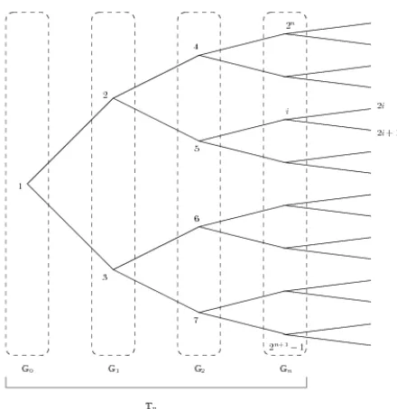
As explained in the introduction, one can see this BAR(p) process as a pth-order autoregressive process on a binary tree, where each vertex represents an individual or cell, vertex 1 being the original ancestor, see Figure 1 for an illustration. For alln_≥1, denote thenth generation by

Figure 1: The tree associated with the bifurcating auto-regressive process.

In particular,G₀ = _{1_} is the initial generation andG₁ =_{2, 3_} is the first generation of offspring from the first ancestor. LetG_r

n be the generation of individual n, which means that rn =log2(n).

Recall that the two offspring of individualnare labelled 2nand 2n+1, or conversely, the mother of individualnis[n/2]. More generally, the ancestors of individual nare[n/2],[n/22], . . . , [n/2rn_].

Furthermore, denote by

T_n=

n [

k=0 G_k

the sub-tree of all individuals from the original individual up to the nth generation. It is clear that the cardinality _|G_n| of G_n is 2n while that of T_n is _|T_n| = 2n+1₋1. Finally, we denote by

T_n,p=_{k∈T_n,k≥2p}the sub-tree of all individuals up to the nth generation withoutT_p−1. One can observe that, for alln_≥1,T_n,0=T_nand, for allp_≥1,T_p,p=G_p.

3

Least-squares estimation

The BAR(p) process (2.1) can be rewritten, for alln≥2p−1, in the matrix form

Z_n=θtY_n+V_n (3.1)

where

Zn= ‚

X_2n X_2n+1

Œ

, Yn= ‚

1

X_n

Œ

, Vn= ‚

ǫ_2n ǫ_2n+1

Œ

and the(p+1)_×2 matrix parameterθ is given by

Our goal is to estimate θ from the observation of all individuals up to the nth generation that is the complete sub-treeT_n. Each new generationG_n contains half the global available information. Consequently, we shall show that observing the whole treeT_n or only generationG_n is almost the same. We propose to make use of the standard LS estimatorθb_nwhich minimizes

∆_n(θ) =1

Consequently, we obviously have for alln_≥p

b

In the special case wherep=1,S_nsimply reduces to

Sn=

In order to avoid useless invertibility assumption, we shall assume, without loss of generality, that for alln≥p−1,Sn is invertible. Otherwise, we only have to add the identity matrix Ip+1 toSn. In

all what follows, we shall make a slight abuse of notation by identifyingθ as well asθb_nto

vec(θ) =

The reason for this change will be explained in Section 4. Hence, we readily deduce from (3.2) that

where_⊗stands for the matrix Kronecker product. Consequently, it follows from (3.1) that

b

θ_n−θ = (I2⊗Sn−−11)

X

k∈T

n−1,p−1

vec€YkVkt Š

= (I_2⊗S_n−₋1₁) X

k∈T_n

−1,p−1

    

ǫ_2k ǫ_2kX_k

ǫ_2k+1 ǫ_2k+1X_k

   

. (3.3)

Denote byF= (_Fn)the natural filtration associated with the BAR(p) process, which means that_Fn is theσ-algebra generated by all individuals up to thenth generation, Fn =σ{Xk,k∈Tn}. In all

the sequel, we shall make use of the five following moment hypotheses.

(H.1) One can findσ2>0 such that, for alln_≥p₋1 and for allk_∈G_n+1,ǫ_kbelongs toL2with

E[ǫ_k|Fn] =0 and E[ǫ_k2_|Fn] =σ2 a.s.

(H.2) It exists _|ρ_| < σ2 such that, for alln≥ p−1 and for all different k,l ∈G_n+1 with[k/2] = [l/2],

E[ǫ_kǫ_l|Fn] =ρ a.s.

Otherwise,ǫ_k andǫ_l are conditionally independent given_Fn.

(H.3) For alln_≥p₋1 and for allk_∈G_n+1,ǫ_kbelongs toL4and

sup

n≥p−1

sup

k∈G_n+1

E[ǫ_k4_|Fn]<_∞ a.s.

(H.4) One can findτ4>0 such that, for alln≥p−1 and for allk∈G_n+1,

E[ǫ_k4_|Fn] =τ4 a.s.

and, forν2< τ4and for all differentk,l_∈G_n+1 with[k/2] = [l/2]

E[ǫ₂2_kǫ₂2_k+1|Fn] =ν2 a.s.

(H.5) For alln_≥p₋1 and for allk_∈G_n+1,ǫ_kbelongs toL8with

sup

n≥p−1

sup

k∈G

n+1

E[ǫ_k8_|Fn]<_∞ a.s.

We now turn to the estimation of the parametersσ2andρ. On the one hand, we propose to estimate the conditional varianceσ2by

b

σ2_n= 1

2|T_n−1|

X

k∈T_n

−1,p−1

kVb_kk2= 1

2|T_n−1|

X

k∈T_n

−1,p−1

(ǫ_b22_k+ǫ_b22_k+1) (3.4)

where for alln_≥p₋1 and for allk_∈G_n,Vb_kt= (ǫ_b2k,ǫ_b2k+1)with

  

b

ǫ_2k = X_{2k −} ba_{0,n −} Pp_i=1ba_i,nX_[ k 2i−1],

b

ǫ_2k+1 = X_{2k+1 −} bb_{0,n −} Pp_i=1bb_i,nX_[ k 2i−1]

.

One can observe that, on the above equations, we make use of only the past observations for the estimation of the parameters. This will be crucial in the asymptotic analysis. On the other hand, we estimate the conditional covarianceρby

b

ρ_n= 1

|T_n−1|

X

k∈T_n

−1,p−1

b

ǫ_2kǫb_2k+1. (3.5)

4

Martingale approach

In order to establish all the asymptotic properties of our estimators, we shall make use of a martin-gale approach. It allows us to impose a very smooth restriction on the driven noise(ǫ_n)compared with the previous results in the literature. As a matter of fact, we only assume suitable moment conditions on(ǫ_n)and that(ǫ_2n,ǫ_2n+1) are conditionally independent, while it is assumed in[14]

that(ǫ_2n,ǫ_2n+1)is a sequence of independent identically distributed random vectors. For alln_≥p, denote

M_n= X

k∈T_n

−1,p−1

    

ǫ_2k ǫ_2kX_k ǫ_2k+1 ǫ_2k+1X_k

    ∈R

2(p+1)_.

LetΣ_n=I_2⊗S_n, and note thatΣ_n−1=I_2⊗S_n−1. For alln_≥p, we can thus rewrite (3.3) as

b

θ_n−θ= Σ−_n−1₁Mn. (4.1)

The key point of our approach is that(M_n)is a martingale. Most of all the asymptotic results for martingales were established for vector-valued martingales. That is the reason why we have chosen to make use of vector notation in Section 3. In order to show that(M_n) is a martingale adapted to the filtration F= (_Fn), we rewrite it in a compact form. Let Ψ_n = I_2⊗Φ_n, where Φ_n is the rectangular matrix of dimension(p+1)_×δ_n, withδ_n=2n, given by

Φ_n= 1 1 · · · 1 X₂n X₂n₊₁ · · · X₂n+1₋₁

!

It contains the individuals of generationsG_n−p+1up toG_nand is also the collection of allY_k,k_∈G_n. Letξ_n be the random vector of dimensionδ_n

ξ_n=

             

ǫ₂n ǫ₂n₊₂

.. .

ǫ₂n+1₋₂ ǫ₂n₊₁ ǫ₂n₊₃

.. .

ǫ₂n+1₋₁

             

.

The vectorξ_ngathers the noise variables of generationG_n. The special ordering separating odd and even indices is tailor-made so thatMn can be written as

Mn= n X

k=p

Ψ_k−1ξ_k.

By the same token, one can observe that

Sn= n X

k=p−1

Φ_kΦt_k and Σ_n=

n X

k=p−1 Ψ_kΨt_k.

Under (H.1) and (H.2), we clearly have for alln_≥0,E[ξ_n+1|Fn] =0 andΨnisFn-measurable. In

addition, it is not hard to see that for alln_≥0,E[ξ_n+1ξt_n+1|Fn] = Γ_⊗I_δ

n whereΓis the covariance

matrix associated with(ǫ_2n,ǫ_2n+1)

Γ = σ 2 _ρ

ρ σ2

!

.

We shall also prove that(Mn) is a square integrable martingale. Its increasing process is given for

alln_≥p+1 by

<M>_n=

n−1

X

k=p−1

Ψ_k(Γ_⊗Iδk)Ψ

t

k= Γ⊗

n−1

X

k=p−1

Φ_kΦt_k= Γ_⊗S_n−1.

It is necessary to establish the convergence ofS_n, properly normalized, in order to prove the asymp-totic results for the BAR(p) estimatorsθb_n,σ_bn2 andρ_bn. One can observe that the sizes ofΨ_n andξ_n

are not fixed and double at each generation. This is why we have to adapt the proof of vector-valued martingale convergence given in[4]to our framework.

5

Main results

Proposition 5.1. Assume that(ǫ_n)satisfies(H.1)to(H.3). Then, we have

lim

n→∞

Sn

|T_n| =L a.s. (5.1)

where L is a positive definite matrix specified in Section 7.

This result is the keystone of our asymptotic analysis. It enables us to prove sharp asymptotic properties for(M_n).

Theorem 5.1. Assume that(ǫ_n)satisfies(H.1)to(H.3). Then, we have

M_ntΣ−_n−1₁Mn=O(n) a.s. (5.2)

In addition, we also have

lim

n→∞

1 n

n X

k=p

M_ktΣ−_k−11 Mk=2(p+1)σ2 a.s. (5.3)

Moreover, if(ǫ_n)satisfies(H.4)and(H.5), we have the central limit theorem

1

p

|T_n−1|

M_{n−→ N}

L

(0,Γ_⊗L). (5.4)

From the asymptotic properties of(Mn), we deduce the asymptotic behavior of our estimators. Our

first result deals with the almost sure asymptotic properties of the LS estimatorθb_n.

Theorem 5.2. Assume that(ǫ_n)satisfies(H.1)to(H.3). Then,θb_n converges almost surely toθ with the rate of convergence

kθb_n−θ _k2=_O

_log

|T_n−1|

|T_n−1|

a.s. (5.5)

In addition, we also have the quadratic strong law

lim

n→∞

1 n

n X

k=1

|T_k−1|(θb_k−θ)tΛ(θb_k−θ) =2(p+1)σ2 a.s. (5.6)

whereΛ =I_2⊗L.

Our second result is devoted to the almost sure asymptotic properties of the variance and covariance estimatorsσ_b2_n andρ_bn. Let

σ2_n= 1

2|T_n−1|

X

k∈T_n

−1,p

(ǫ2_2k+ǫ₂2_k+1) and ρ_n= 1

|T_n−1|

X

k∈T_n

−1,p

ǫ_2kǫ_2k+1.

Theorem 5.3. Assume that (ǫ_n) satisfies (H.1)to (H.3). Then, σb2_n converges almost surely to σ2. More precisely,

lim

n→∞

1

n

X

k∈T_n

−1,p

lim

n→∞

|T_n|

n (σb

2

n−σ

2

n) =2(p+1)σ

2 _{a.s. (5.8)}

In addition,ρb_n converges almost surely toρ

lim

n→∞

1 n

X

k∈T_n−1,p

(ǫ_b2k−ǫ_2k)(ǫ_b2k+1−ǫ_2k+1) = (p+1)ρ a.s. (5.9)

lim

n→∞

|T_n|

n (ρbn−ρn) =2(p+1)ρ a.s. (5.10)

Our third result concerns the asymptotic normality for all our estimatorsθb_n,σ_b2_nandρ_bn.

Theorem 5.4. Assume that(ǫ_n)satisfies(H.1)to(H.5). Then, we have the central limit theorem

p

|T_n−1|(θb_n−θ)_{−→ N}

L

(0,Γ_⊗L−1). (5.11)

In addition, we also have

p

|T_n−1|(σ_bn2₋σ2)_{−→ N}

L

0,τ

4

−2σ4+ν2

2

(5.12)

and

p

|T_n−1|(ρ_bn−ρ)_{−→ N}

L

(0,ν2₋ρ2). (5.13)

The rest of the paper is dedicated to the proof of our main results. We start by giving laws of large numbers for the noise sequence(ǫ_n)in Section 6. In Section 7, we give the proof of Proposition 5.1. Sections 8, 9 and 10 are devoted to the proofs of Theorems 5.2, 5.3 and 5.4, respectively. The more technical proofs, including that of Theorem 5.1, are postponed to the Appendices.

6

Laws of large numbers for the noise sequence

We first need to establish strong laws of large numbers for the noise sequence(ǫ_n). These results will be useful in all the sequel. We will extensively use the strong law of large numbers for locally square integrable real martingales given in Theorem 1.3.15 of[4].

Lemma 6.1. Assume that(ǫ_n)satisfies(H.1)and(H.2). Then

lim

n→+∞

1 |T_n|

X

k∈T_n,p

ǫ_k=0 a.s. (6.1)

In addition, if (H.3)holds, we also have

lim

n→+∞

1 |T_n|

X

k∈T_n,p

ǫ2_k=σ2 a.s. (6.2)

and

lim

n→+∞

1 |T_n−1|

X

k∈T

n−1,p−1

Proof:On the one hand, let

Pn= X

k∈T

n,p ǫ_k=

n X

k=p X

i∈G_k

ǫ_i.

We have

∆Pn+1=Pn+1−Pn= X

k∈G

n+1 ǫ_k.

Hence, it follows from (H.1) and (H.2) that(Pn)is a square integrable real martingale with

increas-ing process

<P>_n= (σ2+ρ)

n X

k=p

|G_k|= (σ2+ρ)(_|T_{n| − |}T_p−1|).

Consequently, we deduce from Theorem 1.3.15 of[4]thatPn=o(<P>n)a.s. which implies (6.1).

On the other hand, denote

Qn= n X

k=p

1 |G_k|

X

i∈G_k ei,

wheree_n=ǫ2_n−σ2. We have

∆Qn+1=Qn+1−Qn=

1 |G_n+1|

X

k∈G_n+1 ek.

First of all, it follows from (H.1) that for allk_∈G_n+1,E[e_k|Fn] =0 a.s. In addition, for all different k,l∈G_n+1 with[k/2]₆= [l/2],

E[e_ke_l|Fn] =0 a.s.

thanks to the conditional independence given by (H.2). Furthermore, we readily deduce from (H.3) that

sup

n≥p−1

sup

k∈G_n+1

E[e2_k|Fn]<∞ a.s.

Therefore,(Q_n)is a square integrable real martingale with increasing process

<Q>_{n ≤} 2 sup

p−1≤k≤n−1

sup

i∈G_k+1

E[e2_i|Fk] n X

j=p

1

|G_j| a.s.

≤ 2 sup

p−1≤k≤n−1

sup

i∈G_k+1

E[e2_i|Fk] n X

j=p ₁

2

j

a.s.

≤ 2 sup

p−1≤k≤n−1

sup

i∈G_k+1

E[e2_i|Fk]<_∞ a.s.

Consequently, we obtain from the strong law of large numbers for martingales that(Q_n)converges almost surely. Finally, as(_|G_n|)is a positive real sequence which increases to infinity, we find from Lemma A.1 in Appendix A that

n X

k=p X

i∈G_k

leading to

Then,(Rn)is a square integrable real martingale which converges almost surely, leading to (6.3). ƒ

Remark 6.2. Note that via Lemma A.2

lim

In fact, each new generation contains half the global available information, observing the whole treeT_n

or only generationG_nis essentially the same.

For the CLT, we will also need the convergence of higher moments of the driven noise(ǫ_n).

Lemma 6.3. Assume that(ǫ_n)satisfies(H.1)to(H.5). Then, we have

Proof : The proof is left to the reader as it follows essentially the same lines as the proof of Lemma 6.1 using the square integrable real martingales

Qn=

Remark 6.4. Note that again via Lemma A.2

7

Proof of Proposition 5.1

Proposition 5.1 is a direct application of the two following lemmas which provide two strong laws of large numbers for the sequence of random vectors(X_n).

Lemma 7.1. Assume that(ǫ_n)satisfies(H.1)and(H.2). Then, we have

lim

n→+∞

1 |T_n|

X

k∈T_n,p

X_k=λ=a(I_p−A)−1e₁ a.s. (7.1)

where a= (a₀+b₀)/2and A is the mean of the companion matrices

A= 1

2(A+B).

Lemma 7.2. Assume that(ǫ_n)satisfies(H.1)to(H.3). Then, we have

lim

n→+∞

1 |T_n|

X

k∈T_n,p

X_kXt

k=ℓ, a.s. (7.2)

where the matrixℓis the unique solution of the equation

ℓ=T+1

2(AℓA

t_+BℓBt₎

T= (σ2+a2_)e 1e1t+

1

2(a0(Aλe

t

1+e1λtAt) +b0(Bλe1t+e1λtBt))

with a2_{= (a}2 0+b

2 0)/2.

Proof : The proofs are given in Appendix A. ƒ

Remark 7.3. We shall see in Appendix A that

ℓ= ∞

X

k=0

1

2k X

C∈{A;B}k C T Ct

where the notation{A;B}kmeans the set of all products of A and B with exactly k terms. For example, we have _{A;B_}0 = _{I_p}, _{A;B_}1 = _{A,B_}, _{A;B_}2 = _{A2,AB,BA,B2_} and so on. The cardinality of {A;B_}k is obviously2k.

Remark 7.4. One can observe that in the special case p=1,

lim

n→+∞

1 |T_n|

X

k∈T

n Xk =

a

1₋b a.s.

lim

n→+∞

1 |T_n|

X

k∈T_n

X_k2 = a

2_+σ2_{+2λa b}

1₋b2 a.s.

where

a b= a0a1+b0b1

2 , b=

a1+b1

2 , b

2₌ a 2 1+b

2 1

8

Proof of Theorems 5.1 and 5.2

Theorem 5.2 is a consequence of Theorem 5.1. The first result of Theorem 5.1 is a strong law of large numbers for the martingale (Mn). We already mentioned that the standard strong law is

useless here. This is due to the fact that the dimension of the random vectorξ_n grows exponentially fast as 2n. Consequently, we are led to propose a new strong law of large numbers for(M_n), adapted to our framework.

Proof of result (5.2) of Theorem 5.1: For all n _≥ p, let _Vn = M_ntΣ−_n−1₁M_n where we recall that

Σ_n=I2⊗Sn, so thatΣ−1n =I2⊗S−1n . First of all, we have

Vn+1 = Mnt+1Σ− 1

n Mn+1= (Mn+ ∆Mn+1)tΣ−n1(Mn+ ∆Mn+1), = M_ntΣ−_n1Mn+2MntΣ−

1

n ∆Mn+1+ ∆Mnt+1Σ− 1

n ∆Mn+1, = _Vn−M_nt(Σ_n−₋1₁₋Σ−_n1)M_n+2M_ntΣ−_n1∆M_n+1+∆Mnt+1Σ−

1

n ∆Mn+1.

By summing over this identity, we obtain the main decomposition

Vn+1+An=Vp+Bn+1+Wn+1, (8.1)

where

An= n X

k=p

M_kt(Σ−_k−1₁₋Σ−_k1)M_k,

Bn+1=2

n X

k=p

M_ktΣ−_k1∆M_k+1 and _Wn+1=

n X

k=p

∆M_kt₊₁Σ−_k1∆M_k+1.

The asymptotic behavior of the left-hand side of (8.1) is as follows.

Lemma 8.1. Assume that(ǫ_n)satisfies(H.1)to(H.3). Then, we have

lim

n→+∞

Vn+1+An

n = (p+1)σ

2 _{a.s. (8.2)}

Proof: The proof is given in Appendix B. It relies on the Riccation equation associated to(S_n)and

the strong law of large numbers for(_Wn). ƒ

Since (_Vn) and(_An) are two sequences of positive real numbers, we infer from Lemma 8.1 that Vn+1=O(n)a.s. which ends the proof of (5.2). ƒ

Proof of result (5.5) of Theorem 5.2:It clearly follows from (4.1) that

Vn= (θbn−θ)tΣn−1(θbn−θ).

Consequently, the asymptotic behavior ofθb_n−θ is clearly related to the one of_Vn. More precisely, we can deduce from convergence (5.1) that

lim

n→∞

λ_min(Σ_n)

since L as well as Λ =I_2⊗L are definite positive matrices. Hereλ_min(Λ)stands for the smallest eigenvalue of the matrixΛ. Therefore, as

kθb_n−θ_k2_≤ Vn λ_min(Σ_n−1),

we use (5.2) to conclude that

kθb_n−θ_k2=_O

_n

|T_n−1|

=_O

_log

|T_n−1|

|T_n−1|

a.s.

which completes the proof of (5.5). ƒ

We now turn to the proof of the quadratic strong law. To this end, we need a sharper estimate of the asymptotic behavior of(_Vn).

Lemma 8.2. Assume that(ǫ_n)satisfies(H.1)to(H.3). Then, we have for allδ >1/2,

kMnk2=o(|Tn−1|nδ) a.s. (8.3)

Proof:The proof is given in Appendix C. ƒ

A direct application of Lemma 8.2 ensures that_Vn=o(nδ)a.s. for allδ >1/2. Hence, Lemma 8.1 immediately leads to the following result.

Corollary 8.3. Assume that(ǫ_n)satisfies(H.1)to(H.3). Then, we have

lim

n→+∞

An

n = (p+1)σ

2 _{a.s. (8.4)}

Proof of result (5.3) of Theorem 5.1:First of all,_Anmay be rewritten as

An= n X

k=p

M_kt(Σ−_k−1₁₋Σ−_k1)M_k=

n X

k=p

M_ktΣ−_k−1/₁2∆_kΣ−_k−1/₁2M_k

where∆_n=I_2(p+1)−Σ1_n−1/2Σ−_n1Σ1_n/₋₁2. In addition, via Proposition 5.1

lim

n→∞

Σ_n

|T_n| = Λ a.s. (8.5)

which implies that

lim

n→∞∆n=

1

2I2(p+1) a.s. (8.6)

Furthermore, it follows from Corollary 8.3 thatAn =O(n)a.s. Hence, we deduce from (8.5) and

(8.6) that

An

n =

  ₂1_n

n X

k=p

M_ktΣ−_k−1₁M_k

 

and convergence (5.3) directly follows from Corollary 8.3. ƒ

We are now in position to prove the QSL.

Proof of result (5.6) of Theorem 5.2: The QSL is a direct consequence of (5.3) together with the fact thatθb_n−θ= Σ−1_n−1M_n. Indeed, we have

1 n

n X

k=p

M_ktΣ−_k−11 Mk =

1 n

n X

k=p

(θb_k−θ)tΣ_k−1(θb_k−θ)

= 1

n

n X

k=p

|T_k−1|(θb_k−θ)t Σk−1

|T_k−1|(θbk−θ)

= 1

n

n X

k=p

|T_k−1|(θb_k−θ)tΛ(θb_k−θ) +o(1) a.s.

which completes the proof of Theorem 5.2. ƒ

9

Proof of Theorem 5.3

The almost sure convergence ofσ_b2_n andρ_bnis strongly related to that of Vb_n−V_n.

Proof of result (5.7) of Theorem 5.3:We need to prove that

lim

n→∞

1 n

X

k∈T_n−1,p−1

kVb_k−V_kk2=2(p+1)σ2 a.s. (9.1)

Once again, we are searching for a link between the sum of_kVb_n−V_nkand the processes(_An)and

(_Vn)whose convergence properties were previously investigated. For alln≥p, we have

X

k∈G_n

kVb_k−V_kk2 = X

k∈G_n

(ǫ_b2k−ǫ_2k)2+ (ǫ_b2k+1−ǫ_2k+1)2,

= (θb_n−θ)tΨ_nΨt_n(θb_n−θ),

= M_ntΣ−_n−1₁Ψ_nΨt_nΣ−_n−1₁M_n,

= M_ntΣ−1_n−/₁2∆_nΣ−1_n−/₁2Mn,

where

∆_n= Σ−_n−1/₁2Ψ_nΨt_nΣ−_n−1/₁2= Σ−_n−1/₁2(Σ_n−Σ_n−1)Σ−_n−1/₁2.

Now, we can deduce from convergence (8.5) that

lim

which implies that

X

k∈G_n

kVb_k−V_kk2=M_ntΣ−1_n−1M_n1+o(1) a.s.

Therefore, we can conclude via convergence (5.3) that

lim

Proof of result (5.8) of Theorem 5.3:First of all,

b

Fn-measurable. Consequently,(Pn)is a real martingale transform. Hence, we can deduce from the

strong law of large numbers for martingale transforms given in Theorem 1.3.24 of[4]together with (9.1) that

It ensures once again via convergence (9.1) that

lim

We now turn to the study of the covariance estimatorρb_n. We have

with

J2=

‚

0 1 1 0

Œ

.

Moreover, one can observe that J2ΓJ2 = Γ. Hence, as before,(Qn) is a real martingale transform

satisfying

Qn=o   

X

k∈T

n−1,p−1

||Vbk−Vk)||2  

=o(n) a.s.

We will see in Appendix D that

lim

n→∞

1 n

X

k∈T_n

−1,p−1

(ǫ_b2k−ǫ_2k)(ǫ_b2k+1−ǫ_2k+1) = (p+1)ρ a.s. (9.2)

Finally, we find from (9.2) that

lim

n→∞

|T_n|

n (ρbn−ρn) =2(p+1)ρ a.s.

which completes the proof of Theorem 5.3. ƒ

10

Proof of Theorem 5.4

In order to prove the CLT for the BAR(p) estimators, we will use the central limit theorem for martingale difference sequences given in Propositions 7.8 and 7.9 of Hamilton[8].

Proposition 10.1. Assume that(W_n)is a vector martingale difference sequence satisfying

(a) For all n≥1,E[W_nW_nt]= Ω_n whereΩ_nis a positive definite matrix and

lim

n→∞

1 n

n X

k=1

Ω_k= Ω

whereΩis also a positive definite matrix.

(b) For all n_≥ 1and for all i,j,k,l, E[W_inW_jnW_knW_{l n}]<_∞ where W_in is the ith element of the vector Wn.

(c)

1 n

n X

k=1

W_kW_kt _−→

P

Ω.

Then, we have the central limit theorem

1 p

n

n X

k=1

We wish to point out that for BAR(p)processes, it seems impossible to make use of the standard CLT for martingales. This is due to the fact that Lindeberg’s condition is not satisfied in our framework. Moreover, as the size of(ξ_n)doubles at each generation, it is also impossible to check condition(c). To overcome this problem, we simply change the filtration. Instead of using the generation-wise filtration, we will use the sister pair-wise one. Let

Gn=σ{X1, (X2k,X2k+1), 1≤k≤n}

be the σ-algebra generated by all pairs of individuals up to the offspring of individual n. Hence

(ǫ_2n,ǫ_2n+1)isGn-measurable. Note thatGn is also theσ-algebra generated by, on the one hand, all

the past generations up to that of individualn, i.e. ther_nth generation, and, on the other hand, all pairs of the(r_n+1)th generation with ancestors less than or equal ton. In short,

Gn=σ

Frn∪ {(X2k,X2k+1), k∈Grn, k≤n}

.

Therefore, (H.2) implies that the processes (ǫ_2n,X_nǫ_2n,ǫ_2n+1,Xnǫ2n+1)t, (ǫ22n+ǫ

2

2n+1−2σ 2_{) and}

(ǫ_2nǫ_2n+1−ρ)are_Gn-martingales.

Proof of result (5.4) of Theorem 5.1: First, recall thatYn= (1,Xn)t. We apply Propositions 10.1

to the_Gn-martingale difference sequence(D_n)given by

D_n=vec(Y_nV_nt) =

    

ǫ_2n X_nǫ_2n

ǫ_2n+1 X_nǫ_2n+1

    .

We clearly have

DnDtn= ‚

ǫ₂2_n ǫ_2nǫ_2n+1 ǫ_2n+1ǫ_2n ǫ2_2n+1

Œ

⊗YnYnt.

Hence, it follows from (H.1) and (H.2) that

E[D_nD_nt] = Γ_⊗E[Y_nY_nt].

Moreover, we can show by a slight change in the proof of Lemmas 7.1 and 7.2 that

lim

n→∞

1 |T_n|

X

k∈T

n−1,p−1

E[DkDkt] = Γ⊗_nlim_→∞

1

|T_n|E[Sn] = Γ⊗L,

which is positive definite, so that condition(a)holds. Condition(b)also clearly holds under (H.3). We now turn to condition(c). We have

X

k∈T_n

−1,p−1

D_kD_kt = Γ_⊗S_n+R_n

where

R_n= X

k∈T_n

−1,p−1

‚

ǫ₂2_k−σ2 ǫ_2kǫ_2k+1−ρ ǫ_2k+1ǫ_2k−ρ ǫ2_2k+1−σ2

Œ

Under (H.1) to (H.5), we can show that(R_n)is a martingale transform. Moreover, we can prove that Rn=o(n)a.s. using Lemma A.6 and similar calculations as in Appendix B where a more complicated

martingale transform(K_n) is studied. Consequently, condition(c) also holds and we can conclude that

1

p

|T_n−1|

X

k∈T_n

−1,p−1

D_k= _p 1

|T_n−1|

M_{n−→ N}

L

(0,Γ_⊗L). (10.1)

Proof of result (5.11) of Theorem 5.4:We deduce from (4.1) that

p

|T_n−1|(θb_n−θ) =_|T_n−1|Σ−_n−1_1pMn

|T_n−1|

.

Hence, (5.11) directly follows from (5.4) and convergence (8.5) together with Slutsky’s Lemma. ƒ

Proof of results (5.12) and (5.13) of Theorem 5.4: On the one hand, we apply Propositions 10.1 to theGn-martingale difference sequence(vn)defined by

vn=ǫ22n+ǫ

2

2n+1−2σ 2_.

Under (H.4), one hasE[v2_n] =2τ4₋4σ4+2ν2which ensures that

lim

n→∞

1 |T_n|

X

k∈T_n,p

−1

E[v_k2] =2τ4₋4σ4+2ν2>0.

Hence, condition(a) holds. Once again, condition(b)clearly holds under (H.5), and Lemma 6.3 together with Remark 6.4 imply condition(c),

lim

n→∞

1 |T_n|

X

k∈T_n,p

−1

v_k2=2τ4₋4σ4+2ν2 a.s.

Therefore, we obtain that

1

p

|T_n−1|

X

k∈T

n−1,p−1

vk=2 p

|T_n−1|(σ2_n−σ2)_{−→ N}

L

(0, 2τ4₋4σ4+2ν2). (10.2)

Furthermore, we infer from (5.8) that

lim

n→∞

p

|T_n−1|(σ_b2_n−σ2_n) =0 a.s. (10.3)

Finally, (10.2) and (10.3) imply (5.12). On the other hand, we apply again Proposition 10.1 to the Gn-martingale difference sequence(wn)given by

wn=ǫ2nǫ2n+1−ρ.

Under (H.4), one hasE[w2_n] =ν2₋ρ2 which implies that condition(a)holds since

lim

n→∞

1 |T_n|

X

k∈T_n,p

−1

Once again, condition(b)clearly holds under (H.5), and Lemmas 6.1 and 6.3 yield condition(c),

lim

n→∞

1 |T_n|

X

k∈T

n,p−1

w2_k=ν2₋ρ2 a.s.

Consequently, we obtain that

1

p

|T_n−1|

X

k∈T_n

−1,p−1

w_k=p_|T_n−1|(ρ_n−ρ)_{−→ N}

L

(0,ν2₋ρ2). (10.4)

Furthermore, we infer from (5.10) that

lim

n→∞

p

|T_n−1|(ρ_bn−ρ_n) =0 a.s. (10.5)

Finally, (5.13) follows from (10.4) and (10.5) which completes the proof of Theorem 5.4. ƒ

Appendices

A

Laws of large numbers for the BAR process

We start with some technical Lemmas we make repeatedly use of, the well-known Kronecker’s Lemma given in Lemma 1.3.14 of[4]together with some related results.

Lemma A.1. Let(α_n)be a sequence of positive real numbers increasing to infinity. In addition, let(x_n)

be a sequence of real numbers such that

∞

X

n=0

|x_n|

α_n <+∞.

Then, one has

lim

n→∞

1

α_n

n X

k=0

x_k=0.

Lemma A.2. Let(x_n)be a sequence of real numbers. Then,

lim

n→∞

1 |T_n|

X

k∈T_n

x_k=x _⇐⇒ lim

n→∞

1 |G_n|

X

k∈G_n

x_k=x. (A.1)

Proof:First of all, recall that_|T_n|=2n+1₋1 and_|G_n|=2n. Assume that

lim

n→∞

1 |T_n|

X

k∈T_n

x_k=x.

We have the decomposition, _X

k∈T_n xk=

X

k∈T_n

−1

xk+ X

Consequently,

A direct application of Toeplitz Lemma given in Lemma 2.2.13 of[4]) yields

lim

In addition, let(X_n)be a sequence of real-valued vectors which converges to a limiting value X . Then,

lim

On the one hand

sup

k≥n−n0

kA_kk and

∞

X

k=n+1

kA_kk

both converge to 0 asntends to infinity. On the other hand,

n X

k=n0+1

kA_{n−kk ≤}

∞

X

n=0

kA_nk<_∞.

Consequently,_kUn−AXkgoes to 0 asngoes to infinity, as expected. ƒ

Lemma A.4. Let(Tn)be a convergent sequence of real-valued matrices with limiting value T . Then,

lim

n→∞

n X

k=0

1

2k X

C∈{A;B}k

C Tn−kCt=ℓ

where the matrix

ℓ= ∞

X

k=0

1

2k X

C∈{A;B}k C T Ct

is the unique solution of the equation

ℓ=T+1

2(AℓA

t_+BℓBt_{). (A.3)}

Proof: First of all, recall that β =max_{kA_k,_kB_k}< 1. The cardinality of_{A;B_}k is obviously 2k. Consequently, if

U_n=

n X

k=0

1

2k X

C∈{A;B}k

C(T_n−k−T)Ct,

it is not hard to see that

kUnk ≤ n X

k=0

1

2k ×2 k_β2k

Tn−k−T =

n X

k=0

β2(n−k)

Tk−T

.

Hence,(U_n)converges to zero which completes the proof of Lemma A.4. ƒ

We now return to the BAR process. We first need an estimate of the sum of the_kX_nk2before being able to investigate the limits.

Lemma A.5. Assume that(ǫ_n)satisfies(H.1)to(H.3). Then, we have

X

k∈T_n,p

Proof:In all the sequel, for alln_≥2p−1, denoteA_2n=AandA_2n+1=B. It follows from a recursive

where

The last two terms of (A.6) are readily evaluated by splitting the sums generation-wise. As a matter of fact,

It remains to control the first termPn. One can observe thatǫkappears inPn as many times as it has

descendants up to thenth generation, and its multiplicative factor for itsith generation descendant is(2β)i. Hence, one has

However, it follows from Remark 6.2 that

lim

In addition, we also have

lim

Consequently, we infer from Lemma A.3 that

Thus,

As before, we deduce from Lemma A.3 that

lim

Finally, Lemma A.5 follows from the conjunction of (A.6), (A.7), (A.8) together with (A.9) and

(A.10). ƒ

Proof of Lemma 7.1 :First of all, denote

Hn=

By induction, we deduce from (A.11) that

H_n

We have already seen via convergence (6.1) of Lemma 6.1 that

it follows from Lemma A.3 that

which ends the proof of Lemma 7.1. ƒ

Proof of Lemma 7.2 : We shall proceed as in the proof of Lemma 7.1 and use the same notation. Let

We infer again from (2.2) that

Kn = Kp−1+

The two first results (6.1) and (6.2) of Lemma 6.1 together with Remark 6.2 and Lemma A.2 readily imply that

In addition, Lemma 7.1 gives

lim

n→+∞

Hn−1

Furthermore, denote it follows from Lemma A.5 that

X

Consequently, we deduce from the strong law of large numbers for martingale transforms given in Theorem 1.3.24 of [4] that Un(u) = o(|Tn|) a.s. for all u∈ Rp which leads to Un = o(|Tn|) a.s.

Therefore, we obtain that(T_n)converges a.s. toT given by

T= (σ2+a2)e1e1t+

Finally, iteration of the recursive relation (A.12) yields

K_n

On the one hand, the first term on the right-hand side converges a.s. to zero as its norm is bounded

β2(n−p+1)_kK_p−1k/2p. On the other hand, thanks to Lemma A.4, the second term on the right-hand side converges toℓgiven by (A.3), which completes the proof of Lemma 7.2. . ƒ

We now state a convergence result for the sum ofkX_nk4which will be useful for the CLT.

Lemma A.6. Assume that(ǫ_n)satisfies(H.1)to(H.5). Then, we have

X

k∈T_n,p

kX_kk4=_O(_|T_n|) a.s. (A.13)

B

On the quadratic strong law

We start with an auxiliary lemma closely related to the Riccation Equation for the inverse of the matrixSn.

Lemma B.1. Let h_nand l_n be the two following symmetric square matrices of orderδ_n

h_n= Φt_nS_n−1Φ_n and l_n= Φ_ntS_n−₋1₁Φ_n.

Then, the inverse of S_n may be recursively calculated as

S_n−1=S−_n−1₁₋S−_n−1₁Φ_n(Iδn+ln) −1_Φt

nS−

1

n−1. (B.1)

In addition, we also have(Iδn−hn)(Iδn+ln) =Iδn.

Remark B.2. If f_n= Ψt_nΣ−_n1Ψ_n, it follows from Lemma B.1 that

Σ−1_n = Σ−1_n−1−Σ−1_n−1Ψ_n(I_2δ

n−fn)Ψ

t

nΣ−1n−1. (B.2)

Proof :AsS_n=S_n−1+ ΦnΦtn, relation (B.1) immediately follows from Riccati Equation given e.g. in [4]page 96. By multiplying both side of (B.1) byΦ_n, we obtain

S−1_n Φ_n = S−1_n−1Φ_n−S−1_n−1Φ_n(I_δ

n+ln) −1_l

n,

= S−_n−1₁Φ_n−S_n−₋1₁Φ_n(Iδn+ln) −1_(I

δn+ln−Iδn), = S−_n−1₁Φ_n(I_δ

n+ln) −1_.

Consequently, multiplying this time on the left byΦ_nt, we obtain that

hn = ln(Iδn+ln) −1_{= (l}

n+Iδn−Iδn)(Iδn+ln) −1_,

= I_δ

n−(Iδn+ln) −1

leading to(I_δ

n−hn)(Iδn+ln) =Iδn. ƒ

In order to establish the quadratic strong law for(Mn), we are going to study separately the

asymp-totic behaviour of(_Wn)and(_Bn)which appear in the main decomposition (8.1).

Lemma B.3. Assume that(ǫ_n)satisfies(H.1)to(H.3). Then, we have

lim

n→+∞

1

nWn=2σ

2 _{a.s. (B.3)}

Proof : First of all, we have the decomposition_Wn+1=_Tn+1+_Rn+1where

Tn+1 =

n X

k=p

∆M_kt₊₁Λ−1∆M_k+1

|T_k| ,

Rn+1 =

n X

k=p

∆M_kt₊₁(_|T_k|Σ_k−1₋Λ−1)∆Mk+1