El e c t ro n ic
Jo ur
n a l o
f P
r o
b a b il i t y
Vol. 13 (2008), Paper no. 68, pages 2069–2106. Journal URL
http://www.math.washington.edu/~ejpecp/
The pattern of genetic hitchhiking under recurrent
mutation
Joachim Hermisson
∗Peter Pfaffelhuber
†Abstract
Genetic hitchhikingdescribes evolution at a neutral locus that is linked to a selected locus. If a beneficial allele rises to fixation at the selected locus, a characteristic polymorphism pattern (so-called selective sweep) emerges at the neutral locus. The classical model assumes that fixation of the beneficial allele occurs from a single copy of this allele that arises by mutation. However, recent theory[Pennings and Hermisson, 2006a,b]has shown that recurrent beneficial mutation at biologically realistic rates can lead to markedly different polymorphism patterns, so-calledsoft selective sweeps. We extend an approach that has recently been developed for the classical hitch-hiking model[Schweinsberg and Durrett, 2005; Etheridge et al., 2006]to study the recurrent mutation scenario. We show that the genealogy at the neutral locus can be approximated (to leading orders in the selection strength) by a marked Yule process with immigration. Using this formalism, we derive an improved analytical approximation for the expected heterozygosity at the neutral locus at the time of fixation of the beneficial allele.
Key words:Selective sweep, genetic hitchhiking, soft selective sweep, diffusion approximation, Yule process, random background.
AMS 2000 Subject Classification:Primary 92D15; Secondary: 60J80, 60J85, 60K37, 92D10. Submitted to EJP on June 11, 2008, final version accepted November 19, 2008.
∗University of Vienna, Nordbergstraße 14, A-1090 Vienna, Austria
email: [email protected]
1
Introduction
The model ofgenetic hitchhiking, introduced by Maynard Smith and Haigh[1974], describes the process of fixation of a new mutation due to its selective advantage. During this fixation process, linked neutral DNA variants that are initially associated with the selected allele willhitchhikeand also increase in frequency. As a consequence, sequence diversity in the neighborhood of the selected locus is much reduced when the beneficial allele fixes, a phenomenon known as a selective sweep. This characteristic pattern in DNA sequence data can be used to detect genes that have been adaptive targets in the recent evolutionary history by statistical tests (e.g. Kim and Stephan 2002; Nielsen et al. 2005; Jensen et al. 2007).
Since its introduction, several analytic approximations to quantify the hitchhiking effect have been developed [Kaplan et al., 1989; Stephan et al., 1992; Barton, 1998; Schweinsberg and Durrett, 2005; Etheridge et al., 2006; Eriksson et al., 2008]. The mathematical analysis of selective sweeps makes use of the coalescent framework[Kingman, 1982; Hudson, 1983], which describes the ge-nealogy of a population sample backward in time. Most studies follow the suggestion of Kaplan et al.
[1989]and use a structured coalescent to describe the genetic footprint at a linked neutral locus, conditioned on an approximated frequency path of the selected allele. In this approach, population structure at the neutral locus consists of the wild-type and beneficial background at the selected lo-cus, respectively. A mathematical rigorous construction was given by Barton et al.[2004]. Moreover, a structured ancestral recombination graph was used in Pfaffelhuber and Studeny[2007]; McVean
[2007]; Pfaffelhuber et al.[2008]to describe the common ancestry of two neutral loci linked to the beneficial allele.
It has long been noted that the initial rise in frequency of a beneficial allele is similar to the evolution of the total mass of a supercritical branching process (Fisher 1930; Kaplan et al. 1989; Barton 1998; Ewens 2004, p. 27f). This insight led to the approximation of the structured coalescent by the genealogy of a supercritical branching process—a Yule process [O’Connell, 1993; Evans and O’Connell, 1994]. Given a selection intensity of α and a recombination rate of ρ between the selected and neutral locus, it has been shown that a Yule process with branching rate α, which is marked at rate ρ and stopped upon reaching ⌊2α⌋ lines, is an accurate approximation of the structured coalescent[Schweinsberg and Durrett, 2005; Etheridge et al., 2006; Pfaffelhuber et al., 2006]. For the standard scenario of genetic hitchhiking, this approach leads to a refined analytical approximation of the sampling distribution, estimates of the approximation error and to efficient numerical simulations.
The paper is organized as follows. In Section 2, we introduce the model as well as the structured coalescent and we discuss the biological context of our work. In Section 3 we state results on the adaptive process, give the approximation of the structured coalescent by a Yule process with immigration and apply the approximation to derive expressions for the heterozygosity at the neutral locus at the time of fixation. In Sections 4, 5 and 6 we collect all proofs.
2
The model
We describe evolution in a two-locus system, where a neutral locus is linked to a locus experiencing positive selection. In Section 2.1, we first focus on the selected locus and formulate the adaptive process as a diffusion. In Section 2.2, we describe the genealogy at the neutral locus by a structured coalescent. In Section 2.3 we discuss the biological context.
2.1
Time-forward process
Consider a population of constant size N. Individuals are haploid; their genotype is thus charac-terized by a single copy of each allele. Selection acts on a single bi-allelic locus. The ancestral (wild-type) allele b has fitness 1 and the beneficial variant B has fitness 1+s, wheres >0 is the selection coefficient. Mutation from btoBis recurrent and occurs with probabilityuper individual per generation. LetXt be the frequency of theBallele in generationt. In a standard Wright-Fisher
model with discrete generations, the number ofB-alleles in the offspring generationt+1 isN Xt+1,
which is binomially distributed with parameters (1+s)Xt+u(1−Xt)
(1+s)Xt+1−Xt andN.
We assume that the beneficial allele B is initially absent from the population in generation t =0 when the selection pressure on the B locus sets in. Since the B allele is created recurrently by mutation and we ignore back-mutations it will eventually fix at some timeT, i.e.Xt=1 fort ≥T. This process of fixation can be approximated by a diffusion. To this end, letXN = (XtN)t=0,1,2,...
withX0N=0 be the path of allele frequencies ofB.
Assumingu=uN →0,s=sN →0 such that 2N u→θ,N s→αasN→ ∞, it is well-known (see e.g. Ewens 2004) that(X⌊N2N t⌋)t≥0⇒(Xt)t≥0 asN→ ∞whereX := (Xt)t≥0 follows the SDE
d X= θ2(1−X) +αX(1−X)d t+pX(1−X)dW (2.1)
withX0=0. In other words, the diffusion approximation ofXN is given by a diffusionX with drift and diffusion coefficients
µα,θ(x) = (θ2 +αx)(1−x), σ2(x) =x(1−x).
We denote byPαp,θ[.]andEpα,θ[.]the probability distribution and its expectation with respect to the diffusion with parametersµα,θ andσ2andX0=palmost surely. The fixation time can be expressed
in the diffusion setting as
2.2
Genealogies
We are interested in the change of polymorphism patterns at a neutral locus that is linked to a se-lected locus. We ignore recombination within the sese-lected and the neutral locus, but (with sexual reproduction) there is the chance of recombination between the selected and the neutral locus. Let the recombination rate per individual beρin the diffusion scaling (i.e. r=rN is the recombination probability in a Wright-Fisher model of sizeN and rN −−−→N→∞ 0 andN rN −−−→N→∞ ρ). Not all recombi-nation events have the same effect, however. We will be particularly interested in events that change the genetic background of the neutral locus at the selected site from B to b, or vice-versa. This is only possible if B individuals from the parent generation reproduce with bindividuals. Under the assumption of random mating, the effective recombination rate in generation t that changes the genetic background is thusρXt(1−Xt)in the diffusion setting.
Following Barton et al. [2004], we use the structured coalescent to describe the polymorphism pattern at the neutral locus in a sample. In this framework, the population is partitioned into two demes according to the allele (B or b) at the selected locus. The relative size of these demes is defined by the fixation path X of the B allele. Only lineages in the same deme can coalesce. Transition among demes is possible by either recombination or mutation at the selected locus. We focus on the pattern at the time T of fixation of the beneficial allele. Throughout we fix a sample sizen.
Remark 2.1. We define the coalescent as a process that takes values in partitions and introduce the following notation. Denote by Σn the set of partitions of {1, ...,n}. Each ξ∈Σn is thus a set
ξ={ξ1, ...,ξ|ξ|}such that
S|ξ|
i=1ξi={1, ...,n}andξi∩ξj=;fori6= j. Partitions can also be defined
by equivalence relations and we writek∼ξℓiff there is 1≤i≤ |ξ|such thatk,ℓ∈ξi. Equivalently,
ξdefines a mapξ:{1, ...,n} → {1, ...,|ξ|}by settingξ(k) =iiffk∈ξi. We will also need the notion
of a composition of two partitions. Ifξis a partition of {1, ...,n}andηis a partition of{1, ...,|ξ|}, define the partitionξ◦ηon{1, ...,n}byk∼ξ◦ηℓiffξ(k)∼ηξ(ℓ).
Settingβ=T−twe are interested in the genealogical processξX = (ξβ)0≤β≤T of a sample of size
n, conditioned on the pathX of the beneficial alleleB. The state space ofξX is
Sn:={(ξB,ξb):ξB∪ξb∈Σn}.
Elements of ξB (ξb) are ancestral lines of neutral loci that are linked to a beneficial (wild-type) allele. Since there are only beneficial alleles at timeT, the starting configuration ofξX is
ξX0 = ({1}, ...,{n},;).
For a given coalescent state ξXβ = (ξB,ξb) at time β, several events can occur, with rates that
depend on the value of the frequency pathX at that time, XT−β. Coalescences of pairs of lines in
the beneficial (wild-type) background occur at rate 1/XT−β (1/(1−XT−β)). Formally, for all pairs 1≤i< j≤ |ξB|and 1≤i′< j′≤ |ξb|, transitions occur at timeβto
(ξB\ {ξBi,ξBj})∪ {ξBi ∪ξBj},ξb with rate 1 XT−β
ξB,(ξb\ {ξib′,ξbj′})∪ {ξbi′∪ξbj′}
with rate 1
1−XT−β
.
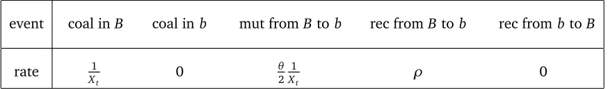
event coal inB coal inb mut fromBto b rec fromBtob rec frombtoB
rate X1
t
1 1−Xt
θ
2 1−Xt
[image:5.612.80.517.92.155.2]Xt ρ(1−Xt) ρXt
Table 1: Transition rates in the processξX at time t = T−β. Coalescence rates are equal for all pairs of partition elements in the beneficial and wild-type background. Recombination and mutation rates are equal for all partition elements inξB andξb.
Changes of the genetic background happen either due to mutation at the selected locus or recom-bination events between the selected and the neutral locus. For 1≤i≤ |ξB|, transitions of genetic backgrounds due to mutation occur at timeβfromξXβ = (ξB,ξb)for 1≤i≤ |ξB|to
ξB\ {ξBi},ξb∪ {ξBi} with rate θ 2
1−XT−β XT−β
. (2.4)
(Recall that we assume that there are no back-mutations to the wild-type). Moreover, changes of the genetic background due to recombination occur at timeβ for 1≤ i≤ |ξB|, 1≤i′≤ |ξb|from
ξXβ = (ξB,ξb)to
ξB\ {ξBi},ξb∪ {ξiB} with rate ρ(1−XT−β) (2.5a)
ξB∪ {ξib′},ξb\ {ξib′}
with rate
ρXT−β. (2.5b)
All rates ofξX are collected in Table 1.
Remark 2.2.
1. The rates for mutation and recombination can be understood heuristically. AssumeXtN = x and assumeu,s,r are small. A neutral locus linked to a beneficial allele in generation t+1 falls into one of three classes: (i) the class for which the ancestor of the selected allele was beneficial has frequencyx+O(u,s,r); (ii) the class for which the beneficial allele was a wild-type and mutated in the last generation has frequency u(1− x) +O(us,ur); (iii) the class for which the neutral locus was linked to a wild-type allele in generation t and recombined with a beneficial allele has frequencyr x(1−x) +O(ru,rs)). Hence, if we are given a neutral locus in the beneficial background, the probability that its linked selected locus experienced a mutation one generation ago isu(1x−x)+O(u2,us,ur)and that it recombined with a wild-type allele one generation ago is r x(1−x)
x +O(ru,rs,r
2). Thus, the rates (2.4) and (2.5a) arise by a
rescaling of time byN.
2.3
Biological context
A selective sweep refers to the reduction of sequence diversity and a characteristic polymorphism pattern around a positively selected allele. Models show that this pattern is most pronounced close to the selected locus if selection is strong and if the sample is taken in a short time window after the fixation of the beneficial allele (i.e. before it is diluted by new mutations). Today, biologists try to detect sweep patterns in genome-wide polymorphism scans in order to identify recent adaptation events (e.g. Harr et al., 2002; Ometto et al., 2005; Williamson et al., 2005).
The detection of sweep regions is complicated by the fact that certain demographic events in the history of the population (in particular bottlenecks) can lead to very similar patterns. Vice-versa, also the footprint of selection can take various guises. In particular, recent theory shows that the pattern can change significantly if the beneficial allele at the time of fixation traces back to more than a single origin at the start of the selective phase (i.e. there is more than a single ancestor at this time). As a consequence, genetic variation that is linked to any of the successful origins of the beneficial allele will survive the selective phase in proximity of the selective target and the reduction in diversity (measured e.g. by the number of segregating sites or the average heterozygosity in a sample) is less severe. Pennings and Hermisson [2006a] therefore called the resulting pattern a soft selective sweepin distinction of the classicalhard sweepfrom only a single origin. Nevertheless, also a soft sweep has highly characteristic features, such as a more pronounced pattern oflinkage disequilibriumas compared to a hard sweep[Pennings and Hermisson, 2006b].
Soft sweeps can arise in several biological scenarios. For example, multiple copies of the beneficial allele can already segregate in the population at the start of the selective phase (adaptation from standing genetic variation; Hermisson and Pennings 2005; Przeworski et al. 2005). Most naturally, however, the mutational process at the selected locus itself may lead to a recurrent introduction of the beneficial allele. Any model, like the one in this article, that includes an explicit treatment of the mutational process will therefore necessarily also allow for soft selective sweeps. For biological ap-plications the most important question then is: When are soft sweeps from recurrent mutation likely? The results of Pennings and Hermisson[2006a] as well as Theorem 1 in the present paper show that the probability of soft selective sweeps is mainly dependent on the population-wide mutation rateθ. The classical results of ahard sweepare reproduced in the limit θ →0 and generally hold as a good approximation forθ <0.01 in samples of moderate size. For largerθ, approaching unity, soft sweep phenomena become important.
Sinceθ scales like the product of the (effective) population size and the mutation rate per allele, soft sweeps become likely if either of these factors is large. Very large population sizes are primarily found for insects and microbial organisms. Consequently, soft sweep patterns have been found, e.g., inDrosophila[Schlenke and Begun, 2004]and in the malaria parasitePlasmodium falsiparum[Nair et al., 2007]. Since point mutation rates (mutation rates per DNA base per generation per individ-ual) are typically very small (∼ 10−8), large mutation rates are usually found in situations where many possible mutations produce the same (i.e. physiologically equivalent) allele. This holds, in particular, for adaptive loss-of-function mutations, where many mutations can destroy the function of a gene. An example is the loss of pigmentation inDrosophila santomea[Jeong et al., 2008]. But also adaptations in regulatory regions often have large mutation rates and can occur recurrently. A well-known example is the evolution of adult lactose tolerance in humans, where several mutational origins have been identified[Tishkoff et al., 2007].
allow for the possibility of back-mutations from the beneficial to the wild-type allele in natural populations. However, such events are rarely seen in any sample because such back-mutants have lower fitness and are therefore less likely to contribute any offspring to the population at the time of fixation. Another step towards a more realistic modeling of genetic hitchhiking under recurrent mutation would be to allow for beneficial mutation to the same (physiological) allele at multiple different positions of the genome. In such a model, recombination between the different positions of the beneficial mutation in the genome would complicate our analysis.
3
Results
The process of fixation of the beneficial allele is described by the diffusion (2.1). In Section 3.1, we will derive approximations for the fixation time T of this process. These results will be needed in Section 3.2, where we construct an approximation for the structured coalescentξX.
3.1
Fixation times
In the study of the diffusion (2.1) the time T of fixation of the beneficial allele (see (2.2)) is of particular interest. We decompose the interval [0;T] by the last time a frequency of Xt =0 was reached, i.e., we define
T0:=sup{t≥0 :Xt=0}, T∗:=T−T0.
Note that forθ ≥1, the boundary x =0 is inaccessible, such thatT0=0,T∗=T, almost surely, in
this case.
Proposition 3.1. 1. Letγe≈0.57be Euler’sγ. Forθ >0,
E0α,θ[T] = 1
α
2 log(2α) +2γe+
1
θ −θ
∞
X
n=1
1 n(n+θ)
+Ologα
α2
+ 1
θO αe
−α (3.1)
2. Forθ≥1, almost surely, T=T∗.
3. For0≤θ≤1,
E0α,θ[T∗] = 2
α log(2α) +γe
+
Ologα
α2
(3.2)
4. Forθ≥0,
V0α,θ[T∗] =O 1
α2
. (3.3)
All error terms are in the limit for largeαand are uniform on compacta inθ.
Remark 3.2.
1. Note that (3.1) reduces to (3.2) forθ=1 as it should since T0
2. Forθ ≤1, we find that E0α,θ[T∗]is independent ofθ to the order considered. In particular it is identical to the conditioned fixation time without recurrent mutation (θ = 0) that was previously derived[van Herwaarden and van der Wal, 2002; Hermisson and Pennings, 2005; Etheridge et al., 2006]. A detailed numerical analysis (not shown) demonstrates that the pas-sage times of the beneficial allele decrease at intermediate and high frequencies, but increase at low frequenciesX®1/αwhere recurrent mutation prevents the allele from dying out. Both effects do not affect the leading order and precisely cancel in the second order for largeα.
3. To leading order in 1/θ andα, the total fixation time (3.1) is
E0α,θ[T]≈ 1
αθ +E
0
α,θ[T∗].
Since the fixation probability of a new beneficial mutation is Pfix ≈ 2s and the rate of new beneficial mutations per time unit (of N generations) is Nθ /2, mutations that are destined for fixation enter the population at ratesNθ =αθ. The total fixation time thus approximately decomposes into the conditioned fixation timeE[T∗]and the exponential waiting time for the establishment of the beneficial allele αθ1 .
4. In applications, selective sweeps are found withα≥100. We can then ignore the error term
1
θO αe−
α/2in (3.1) even for extremely rare mutations withθ
∼10−10.
5. The proof of Proposition 3.1 can be found in Section 4.
3.2
The Yule approximation
We will provide a useful approximation of the coalescent process with rates defined in (2.3)–(2.5). As already seen in the last section the process of fixation of the beneficial allele can be decomposed into two parts. First, the beneficial allele has to be established, i.e., its frequency must not hit 0 any more. Second, the established allele must fix in the population. The first phase has an expected length of about 1/(αθ) and hence may be long even for large values ofα, depending onθ. The second phase has an expected length of order(logα)/αand is thus short for largeα, independently of θ. For the potentially long first phase we give an approximation for the distribution of the coalescent on path space by a finite Kingman coalescent. For the short second phase, we obtain an approximation of the distribution of the coalescent (which is started at time T) at time T0 using a Yule process with immigration (which constructs a genealogy forward in time). To formulate our results, define
β0:=T−T0.
Setting Xt =0 for t <0 we will obtain approximations for the distribution of coalescent states at timeβ0,
ξβ0:= (ξ
B
β0,ξ
b
β0):=
Z
Pα,θ[dX]ξXβ
0,
and of the genealogies forβ > β0, i.e. in the phase prior to establishment of the beneficial allele,
ξ≥β0:= (ξ
B
≥β0,ξ
b
≥β0):=
Z
t
pr
es
ent
pa
st
1 23 4 65
2
αα
lines
recombination
recomb.
[image:9.612.124.460.113.298.2]mutation
Figure 1: The Yule process approximation for the genealogy at the neutral locus in a sample of sizen=6. The Yule process with immigration produces a random forest (grey lines) which grows from the past (past) to the present (top). A sample is drawn in the present. Every line is marked at constant rate along the Yule forest indicating recombination events. Sample individuals within the same tree not separated by a recombination mark share ancestry and thus belong to the same partition element ofΥ. In this realization, we findΥ ={{1},{2, 3},{4},{5, 6}}.
Note thatξβ0∈Sn whileξ≥β0 ∈ D([0;∞),Sn), the space of cadlag paths on[0;∞)with values in Sn.
Let us start withξβ0 (see Figure 1 for an illustration of our approximation). Consider the selected
site first. Take a Yule process with immigration. Starting with a single line,
• every line splits at rateα.
• new lines (mutants) immigrate at rateαθ.
For this process we speak of Yule-time ifor the time the Yule process hasi lines for the first time. We stop this Yule process with immigration at Yule-time⌊2α⌋. In order to define identity by descent within a sample ofnlines, take a sample ofnrandomly picked lines from the⌊2α⌋. Note that the Yule process with immigration defines a random forestF and we may define the random partition
e
Υof{1, ...,n}by saying that
k∼Υe ℓ ⇐⇒ k,ℓare in the same tree ofF.
As a special case of Theorem 1 we will show thatΥe is a good approximation toξβ0in the caseρ=0.
at time T0, which carries the wild-type allele. Since recombination events take place with a rate proportional toρandT−T0=T∗is of the order(logα)/α, it is natural to use the scaling
ρ=γ α
logα. (3.4)
Take a sample ofnlines from the⌊2α⌋lines of the top of the Yule tree and consider the subtree of thenlines. Indicating recombination events, we mark all branches in the subtree independently. A branch in the subtree, which starts at Yule-timei1and ends at Yule-timei2is marked with probability
1−pi2
i1(γ,θ), where
pi2
i1(γ,θ):=exp
−logγ
α
i2
X
i=i1+1
1 i+θ
. (3.5)
Then, define the random partitionΥof{1, ...,n}(our approximation ofξβ0) by
k∼Υℓ ⇐⇒ k∼Υe ℓ ∧ path fromktoℓinF not separated by a mark.
To obtain an approximation ofξ≥β0 consider the finite Kingman coalescent C := (Ct)t≥0. Given
there aremlines such thatCt=C={C1, ...,Cm}, transitions occur for 1≤1< j≤mto
C\ {Ci,Cj}∪ {Ci∪Cj}with rate 1.
GivenΥ, our approximation ofξ≥β0 is
Υ◦ C := (Υ◦Ct)t≥0.
Remark 3.3. Our approximations are formulated in terms of the total variation distance of proba-bility measures. Given two probaproba-bility measuresP,Qon aσ-algebraA, the total variation distance is given by
dT V(P,Q) =12 sup
A∈A|
P[A]−Q[A]|.
Similarly, for two random variablesX,Y onΩwithσ(X) =σ(Y)and distributionsL(X)andL(Y)
we will write
Theorem 1.
1. The distribution of coalescent statesξβ0 at timeβ0 under the full model can be approximated by
a distribution of coalescent states of a Yule process with immigration. In particular,
Pα,θ[ξBβ
0=;] =1 (3.6)
and the bound
dT V ξβb
0,Υ
=O 1
(logα)2
(3.7)
holds in the limit of largeαand is uniform on compacta in n,γandθ.
2. The distribution of genealogies ξ≥β0 prior to the establishment of the beneficial allele can be
approximated by the distribution of genealogies under a composition of a Yule process with immi-gration and the Kingman coalescent. In particular,
P[ξB≥β
06= (;)t≥0] =O
1
αlogα
and the bound
dT V ξ≥bβ0,Υ◦ C
=
O 1
(logα)2
(3.8)
holds in the limit of largeαand is uniform on compacta in n,γandθ.
Remark 3.4.
1. Let us give an intuitive explanation for the approximation of the genealogy at the selected site byΥe. Consider a finite population of sizeN. It is well-known that a supercritical branching process is a good approximation for the frequency path X at times t when Xt is small. In
such a process, each individual branches at rate 1. It either splits in two with probability 1+2s or dies with probability 1−2s. In this setting every line has a probability of 2s+O(s2)≈2α/N to be of infinite descent. In particular, new mutants that have an infinite line of descent arise approximately at rate 2s·N u=αθ /N. In addition, when there are 2N slines of infinite descent there must be approximatelyNlines in total, which is the whole population.
2. Using the approximation of ξβ0 by Υwe can immediately derive a result found in Pennings
3. When biologists screen the genome of a sample for selective sweeps, they can not be sure to have sampled at time t = T. Given they have sampled lines linked to the beneficial type at t<T when the beneficial allele is already in high frequency (e.g. Xt≈1−δ/logαfor some
δ >0), the approximations of Theorem 1 still apply. The reason is that neither recombination events changing the genetical background nor coalescences occur in [t;T] in ξ with high probability; see Section 6.6. If t > T, a good approximation to the genealogy isC ◦e Υ◦ C
whereCeis a Kingman coalescent run for timet−T.
4. The model parameters n,γand θ enter the error terms O(.) above. The most severe error in (3.7) arises from ignoring events with two recombination events on a single line. See also Remark 5.4. Hence,γenters the error term quadratically. Since each line might have a double-recombination history, the sample sizen enters this error term linearly. The contribution of
θ to the error term cannot be seen directly and is a consequence of the dependence of the frequency pathX onθ.
Note that coalescence events always affect pairs of lines while both recombination and muta-tion affects only single lines. As a consequence,nenters quadratically into higher order error terms. In particular, for practical purposes, the Yule process approximation becomes worse for big samples.
5. The proof of Theorem 1 can be found in Section 6. Key facts needed in the proof are collected in Section 5.
3.3
Application: Expected heterozygosity
The approximation of Theorem 1 using a Yule forest as a genealogy has direct consequences for the interpretation of population genetic data. While genealogical trees cannot be observed directly, their impact on measures of DNA sequence diversity in a population sample can be described. The idea is that mutations along the genealogy of a sample produce polymorphisms that can be observed. Genealogies in the neighbourhood of a recent adaptation event are shorter, on average, meaning that sequence diversity is reduced. This reduction is stronger, however, for a ’hard sweep’ (see Section 2.3), where the sample finds a common ancestor during the time of the selective phase E[T∗]≈
2 log(α)/α≪1 than for a ’soft sweep’, where the most recent common ancestor is older. Using our fine asymptotics for genealogies, we are able to quantify the prediction of sequence diversity under genetic hitchhiking with recurrent mutation. In this section we will concentrate on heterozygosity as the simplest measure of sequence diversity.
By definition, heterozygosity is the probability that two randomly picked lines from a population are different. WritingHt for the heterozygosity at timet and using (3.6), we obtain
HT =Pα,θ[ξβb0={{1},{2}}|ξ0= ({1},{2},;)]·HT0.
Assuming that the population was in equilibrium at time 0, we can use Theorem 1, in particular (3.7), to obtain an approximation for the heterozygosity at timeT.
Proposition 3.5. Abbreviating pi:=pi⌊2α⌋(γ,θ)(compare(3.5)), heterozygosity at time T is approxi-mated by
HT HT0 =1−
p21
θ+1− 2γ
logα
⌊X2α⌋
i=2
2i+θ
(i+θ)2(i+1+θ)p 2
i +O
1
(logα)2
1 2 5 10 20 50 100 200 500
0.0
0.2
0.4
0.6
0.8
1.0
ρρ
HT HT
0
θθ=0
θθ=0.4
θθ=1
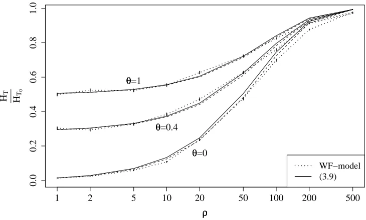
[image:13.612.109.474.102.322.2]WF−model (3.9)
Figure 2: Reduction in heterozygosity at time of fixation of the beneficial allele. The x-axis shows the recombination distance of the selected from the neutral locus. Solid lines connect results from the analytical approximation. Dotted lines show simulation results of a structured coalescent in a Wright-Fisher model withN =104 andα=1000. Small vertical bars indicate standard errors from 103 numerical iterations.
where the error is in the limit of largeαand is uniform on compacta in n,γandθ.
Remark 3.6.
1. The formula (3.9) establishes that
HT HT0 =1−
p12
θ+1+O
1
logα
. (3.10)
In particular, to a first approximation, two lines taken from the population at time T are identical by descent if their linked selected locus has the same origin (probability 1+1θ) and if both lines were not hit by independent recombination events (probabilityp21).
2. We investigated the quality of the approximation (3.9) by numerical simulations. The outcome can be seen in Figure 2. As we see, forα=1000, our approximation works well for all values ofθ≤1 up toρ/α=0.1, i.e.,γ=0.7.
3. We can compare Proposition 3.5 with the result for the heterozygosity under a star-like ap-proximation for the genealogy at the selected site, which was used by Pennings and Hermisson
[2006b, eq. (8)], i.e.
HT
HT0
≈1− e −2γ
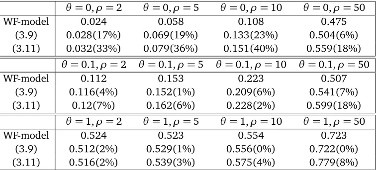
θ=0,ρ=2 θ=0,ρ=5 θ =0,ρ=10 θ=0,ρ=50
WF-model 0.024 0.058 0.108 0.475
(3.9) 0.028(17%) 0.069(19%) 0.133(23%) 0.504(6%)
(3.11) 0.032(33%) 0.079(36%) 0.151(40%) 0.559(18%)
θ=0.1,ρ=2 θ =0.1,ρ=5 θ=0.1,ρ=10 θ=0.1,ρ=50
WF-model 0.112 0.153 0.223 0.507
(3.9) 0.116(4%) 0.152(1%) 0.209(6%) 0.541(7%)
(3.11) 0.12(7%) 0.162(6%) 0.228(2%) 0.599(18%)
θ=1,ρ=2 θ=1,ρ=5 θ =1,ρ=10 θ=1,ρ=50
WF-model 0.524 0.523 0.554 0.723
(3.9) 0.512(2%) 0.529(1%) 0.556(0%) 0.722(0%)
[image:14.612.110.488.90.261.2](3.11) 0.516(2%) 0.539(3%) 0.575(4%) 0.779(8%)
Table 2: Comparison of numerical simulation of a Wright-Fisher model to (3.9) and (3.11). Numbers in brackets are the relative error of the approximation. For θ = 0 and θ = 1, the same set of simulations as in Figure 2 are used. In particular,N =104 andα=1000.
Note that this formula also arises approximately by takingp⌊12α⌋(γ, 0)instead ofp1 in (3.10).
As shown in Table 2, the additional terms from the Yule process approximation lead to an improvement over the simple star-like approximation result.
4. The quantification of sequence diversity patterns for selective sweeps with recurrent mutation using the Yule process approximation is not restricted to heterozygosity. Properties of several other statistics could be computed. As an example, we mention the site frequency spectrum, which describes the number of singleton, doubleton, tripleton, etc, mutations in the sample.
Moreover, as pointed out by Pennings and Hermisson (2006b), selective sweeps with recurrent mutation also lead to a distinct haplotype pattern around the selected site. Intuitively, every beneficial mutant at the selected site brings along its own genetic background leading to several extended haplotypes. Quantifying such haplotypes patterns would require models for more than one neutral locus.
Proof of Proposition 3.5. Using Theorem 1 we have to establish that Pα,θ[ξβb0 = {{1, 2}}|ξ0 =
accounting for all possibilities when coalescence of two lines can occur,
P[Υ ={{1, 2}}] =
⌊X2α⌋
i=1
i i+θ
1
i+1 2
p2i · ⌊Y2α⌋
j=i+1
θ
j+θ
1− 2 j+1
+ j
j+θ
1− j+11
2
=
⌊X2α⌋
i=1
2p2i
(i+θ)(i+1)·
⌊2α⌋
Y
j=i+1
θ j−1
(j+θ)(j+1)+
(j−1)(j+2) (j+θ)(j+1)
=
⌊X2α⌋
i=1
2p2i
(i+θ)(i+1)·
⌊2α⌋
Y
j=i+1
j−1 j+1
j+2+θ
j+θ
=
⌊X2α⌊
i=1
2p2i i+θ
i
(i+1+θ)(i+2+θ)+O
1
α
=
⌊X2α⌋
i=1
2
(i+1+θ)(i+2+θ)−
2θ
(i+θ)(i+1+θ)(i+2+θ)
p2i +O1
α
.
Rewriting gives
P[Υ ={{1, 2}}] =
⌊X2α⌋
i=1
2p2i i+1+θ −
2pi2 i+2+θ
−θ
⌊X2α⌋
i=1
p2i
(i+θ)(i+1+θ)−
p2i
(i+1+θ)(i+2+θ)
+O1
α
= 2p
2 1
θ+2+ ⌊X2α⌋
i=1
2(p2i+1−p2i)
i+2+θ
−θ p
2 1
(θ+1)(θ+2)−θ
⌊2α⌋
X
i=1
p2i+1−p2i
(i+1+θ)(i+2+θ)+O
1 α = p 2 1
θ+1+ ⌊X2α⌋
i=1
2i+θ+2
(i+1+θ)(i+2+θ)(p
2
i+1−p 2
i) +O
1 α = p 2 1
θ+1+ 2γ
logα
⌊X2α⌋
i=2
p2i 2i+θ
(i+θ)2(i+1+θ)+O
1
(logα)2
where the last equality follows from
p2i+1−p2i =p2i+11−exp− 2γ
logα
1 i+1+θ
=p2i+1 2γ logα
1 i+1+θ +
1
i2O
1
(logα)2
4
Proof of Proposition 3.1 (Fixation times)
Our calculations are based on the Green functiont(.; .)for the diffusionX = (Xt)t≥0. This function
satisfies
Eαp,θh Z
T
0
f(Xt)d ti=
Z 1
0
t(x;p)f(x)d x (4.1)
and
Eαp,θh Z
T
0 Z T
t
f(Xt)g(Xs)dsd ti=
Z 1
0 Z 1
0
t(x;p)t(y;x)f(x)g(y)d y d x. (4.2)
Using
ψα,θ(y):=ψ(y):=exp
−2
Z y
1
µα,θ(z)
σ2(z) dz
= 1
yθ exp(2α(1− y))
the Green function forX, started inp, is given by (compare Ewens[2004], (4.40), (4.41))
tα,θ(x;p) = 2
σ2(x)ψ(x) Z 1
x∨p
ψ(y)d y= 2
x(1−x)
Z 1
x∨p
e−2α(y−x)x y
θ
d y.
Since T∗ depends only on the path conditioned not to hit 0, we need the Green function of the conditioned diffusion. To derive its infinitesimal characteristics, we need the absorption probability, i.e., given a current frequency of p of the beneficial allele, its probability of absorption at 1 before hitting 0. This probability is given by
Pα1,θ(p) =
Rp
0 ψ(y)d y R1
0 ψ(y)d y
=
Rp
0
e−2αy yθ d y
R1 0
e−2αy
yθ d y
forθ <1. Forθ ≥1, we havePα1,θ =1, i.e., 0 is an inaccessible boundary. In the caseθ <1, the Green function of the conditioned process is forp≤x (compare Ewens[2004], (4.50))
t∗α,θ(x;p) =Pα1,θ(x)·tα,θ(x;p)
and forx ≤p(see Ewens[2004], (4.49))
t∗α,θ(x;p) = 2
σ2(x)ψ(x)
(1−Pα1,θ(x))Pα1,θ(x)
Pα1,θ(p)
Z x
0
ψ(y)d y
=2 1
σ2(x)ψ(x) R1
pψ(y)d y
Rx
0 ψ(y)d y Rx
0 ψ(y)d y Rp
0 ψ(y)d y R1
0 ψ(y)d y
.
Lemma 4.1. 1. Forǫ,K∈(0;∞)there exists C∈Rsuch that
sup
ǫ≤x≤1,0≤θ≤K
1−x
θ
θ(1−x)
≤C. (4.3)
2. Forθ∈[0; 1),
Z 1
0
z−θe−2αzdz= 1
2α1−θΓ(1−θ) +O(e
−2α) (4.4)
whereΓ(.)is the Gamma function.
3. The bounds
Z 1
0
xθ−1e−2α(1−x)d x=O1
α
+ 1
θO αe
−α, (4.5)
Z 1
0
1−e−2αx
x d x−log 2α+γe=O 1
α
, (4.6)
Z 1
0
1−xθ 1−x e
−2α(1−x)d x= O1
α
, (4.7)
Z 1
0 Z y/2
0
1 1−x
x y
θ
e−2α(y−x)d x d y=O 1
α2
(4.8)
hold in the limit of largeα, and uniformly on compacta inθ.
Proof. 1. By a Taylor approximation of x 7→xθ around x =1 we obtain
xθ =1+θ(1−x) +θ(θ2−1)ξθ−2(1−x)2
for somex ≤ξ≤1 and the result follows.
2. We simply compute
Z 1
0
z−θe−2αzdz= 1 (2α)1−θ
Z 2α
0
e−zz−θdz= 1
(2α)1−θΓ(1−θ) +O(e−
2α) (4.9)
3. For (4.5), we write
Z 1
0
xθ−1e−2α(1−x)d x= 1
θx
θe−2α(1−x) 1
0+
2α θ
Z 1
0
xθe−2α(1−x)d x
= 1
θ −
2α θ
Z 1
0
e−2αxd x+O2θαe−α+2α
Z 1
0
(1−x)e−2α(1−x)d x
=O1
α
+ 1
θO αe
where we have used 1. for ǫ= 12. For (4.6), see[Bronstein, 1982, p. 61]. Equation (4.7) follows from
Z 1
0
1−xθ 1−x e
−2α(1−x)d x ≤
Z 1
0
1−x⌈θ⌉ 1−x e
−2α(1−x)d x=
⌈θ⌉
X
i=0 Z 1
0
xie−2α(1−x)d x≤ ⌈θ⌉
2α
and (4.8) from
Z 1
0 Z y/2
0
1 1−x
x y
θ
e−2α(y−x)d x d y≤2
Z 1
0 Z y/2
0
e−2α(y−x)d x d y
= 1
2α
Z 1
0
e−2αy−e−2αy/2d y=O 1
α2
.
Lemma 4.2. Let2α≥1. There is C>0such that for allθ ∈[0; 1]and x∈[0; 1]
Pα1,θ(x)≤ C(2αx)1−θ∧1.
Proof. By a direct calculation, we find
Pα1,θ(x) =
R2αx
0
e−y
yθ d y
R2α
0
e−y
yθ d y
≤ R2αx
0 y
−θ
R1 0
e−1
yθ
=e·(2αx)1−θ
Moreover, sincePα1,θ(x)is a probability, the boundPα1,θ(x)≤1 is obvious.
Proof of Proposition 3.1. We start with the proof of (3.1), i.e., we set f =1 in (4.1). We split the integral ofEα,θ[T]by using x(11−x)= 1x +1−1x, i.e.,
Eα,θ[T] =2
Z 1 0 Z y 0 1 x x y θ
e−2α(y−x)d x d y+2
Z 1
0 Z y
0
1 1−x
x y
θ
e−2α(y−x)d x d y.
For the first part,
2 Z 1 0 Z y 0 1 x x y θ
e−2α(y−x)d x d y x→=x/y2
Z 1
0 Z 1
0
xθ−1e−2αy(1−x)d y d x
= 1
α
Z 1
0
xθ−1 1
1−x 1−e
−2α(1−x)d x
= 1
α
Z 1
0
xθ−1+ x θ
1−x
1−e−2α(1−x)d x
= 1 α 1 θ − Z 1 0
1−xθ 1−x (1−e
−2α(1−x))d x+ Z 1
0
1−e−2α(1−x) 1−x d x
+O 1
α2
+ 1
θO αe
−α = 1 α 1 θ − ∞ X
n=0 Z 1
0
(xn−xn+θ)d x+log(2α) +γe
+O 1
α2
+ 1
θO 2αe
−α = 1 α 1 θ −θ ∞ X
n=1
1
n(n+θ)+log(2α) +γe
+O 1
α2
+ 1
θO αe
where we have used (4.5) in the fourth and both, (4.6) and (4.7) in the fifth equality. The second part gives, using (4.8) and (4.3),
2 Z 1 0 Z y 0 1 1−x
x y
θ
e−2α(y−x)d x d y=2
Z 1
0 Z y/2
0
1 1−x
x y
θ
e−2α(y−x)d x d y
+2
Z 1
0 Z y/2
0
1 1−y+x
1− x y
θ
e−2αxd x d y
=2 Z 1 0 Z y 0 1 1−y+xe
−2αxd x d y+
O Z 1
0 Z y
0
x 1+x
1
1−y+x + 1 y
e−2αxd x d y+O 1
α2 =2 Z 1 0 Z y 0 1 1−xe
−2α(y−x)d y d x+ O Z
1
0
xlog y
1− y+x
y=1
y=xe
−2αxd x+
O 1
α2 = 1 α Z 1 0
1−e−2α(1−x) 1−x d x+O
1
α2 Z 2α
0
xlog2α x
e−xd x+O 1
α2
= 1
α log 2α+γe
+Ologα
α2
(4.10) and (3.1) follows. For the proof of (3.2) we have
Eα,θ[T∗] =
2R1
0 R1
x
Rx
0
e−2α(y−x)
x(1−x) x
yz
θ
e−2αzdzd y d x R1
0 z−
θe−2αzdz
(4.11)
By using x(11 −x)=
1
x +
1
1−x we again split the integral in the numerator. For the
1
x-part we find
2 Z 1 0 Z 1 x Z x 0
e−2α(y−x) x
x yz
θ
e−2αzdzd y d x x→=x/y2
Z 1
0 Z 1
0 Z x y
0
e−2α(y(1−x)) x
x z
θ
e−2αzdzd y d x
z→z/x
= 2 Z 1 0 Z 1 0 Z y 0
e−2αy(1−x)z−θe−2αz xdzd y d x
= 1 α Z 1 0 Z 1 0 1 1−x e
−2αz(1−x)
−e−2α(1−x)z−θe−2αz xdzd x
1→1−x
= 1 α Z 1 0 Z 1 0 1 x e
−2αz
−e−2α(x+z−xz)z−θdzd x
= 1
α
Z 1
0
1−e−2αx
x d x
Z 1
0
e−2αzz−θdz+ 1
α Z 1 0 Z 1 0 1 xe
−2α(x+z) 1
Using (4.4) we see that Z 1 0 Z 1 0 1 xe
−2α(x+z) e2αxz
−1z−θd x dz=
∞
X
n=1 Z 1
0
e−2αzzn−θdz Z 2α
0
e−xx
n−1
n! d x
=O Z
1
0
e−2αzz−θ ∞
X
n=1
zn ndz
=O Z
1
0
e−2αzz−θlog(1−z)dz
=O Z
1
0
z1−θe−2αzdz
= Γ(2−θ)O 1
α2−θ
(4.12)
such that, with (4.4),
2R01Rx1R0x e−α(xy−x)yzx θe−αzdzd y d x R1
0 z−
θe−αzdz
= 1
α log 2α+γe
+ O 1
α2
. (4.13)
For the 11
−x-part, we write
Z 1 0 Z 1 x Z x 0
e−2α(y−x) 1−x
x yz
θ
e−2αzdzd y d x− Z 1
0
z−θe−2αzdz Z
1
0 Z 1
x
e−2α(y−x) 1−x
x y
θ
d y d x
= Z 1 0 Z 1 x Z 1 x
e−2α(y−x) 1−x
x yz
θ
e−2αzdzd y d x
=O Z
1
0
z−θe−2αz Z z
0 Z 1
x
e−2α(y−x)
1−x d y d x dz
=O1
α
Z 1
0
z−θe−2αz Z 1
1−z
1−e−2αx x d x dz
=O1
α
Z 1
0
z−θe−2αzlog(1−z)dz
=O1
α
Z 1
0
z1−θe−2αzdz
= Γ(2−θ)O 1
α3−θ
where we have used (4.4) in the last step. Hence, by (4.10),
2R1
0 R1
x
Rx
0
e−2α(y−x) 1−x
x
yz
θ
e−2αzdzd y d x R1
0 z−
θe−2αzdz =
1
α log 2α+γe
+θOlogα
α2
+O 1
α2
. (4.14)
For the variance we start withθ <1. By (4.2) and a similar calculation as in the proof of Lemma 4.2, for some finiteC (which is independent ofθ andα), using (4.2)
V0[T∗] =2
Z 1
0 Z w
0
t∗θ(w; 0)tθ∗(x;w)d x d w
=4
Z 1
0 Z w
0
e2α(w+x) w1−θ(1
−w)x1−θ(1
−x)
Z 1
w
e−2αy yθ d y
Z1
w
e−2αz zθ dz
R0x e−2αˆz ˆ
zθ dˆz
R1 0
e−2α˜z ˜
zθ d˜z
2
d x d w
w,x,y,z→
≤ 2α(w,x,y,z)
C
α2 Z 2α
0 Z w 0 Z 1 w Z 1 w
ew+x−y−z w(1−2wα)x(1−2xα)
w x yz
θ
(x2−2θ ∧1)dzd y d x d w
= 2C
α2 Z 2α
0 Z z 0 Z y 0 Z w 0 1 w + 1 2α−w
1
x + 1 2α−x
ew+x−y−zw x yz
θ
(x2−2θ ∧1)d x d wd y dz
(4.15) where the last equality follows by the symmetry of the integrand with respect to y andz. We divide the last integral into several parts. Moreover, we use that
Z 2α
0 Z z 0 Z y 0 Z w 0
...d x d wd y dz=
Z 2α
0 Z z
0 Z y
0 Z w∧1
0
...d x d wd y dz+
Z 2α
1 Z z 1 Z y 1 Z w 1
...d x d wd y dz.
(4.16)
First,
Z 2α
0 Z z 0 Z y 0 Z w 0 1 w xe
w+x−y−zw x
yz θ
(x2−2θ∧1)d x d wd y dz
=O Z
∞ 0 Z z 0 Z y 0 Z w∧1
0
e−z w x
w x yz
θ
x2−2θd x d wd y dz+
Z ∞ 1 Z z 1 Z y 1 Z w 1
ew+x−y−z
w x d x d wd y dz
=O 1
2−θ
Z ∞ 0 Z z 0 Z y 0
e−zw 1 yz
θ
d wd y dz+
Z ∞ 1 Z ∞ x Z ∞ w Z ∞ y
ew+x−y−z
w x dzd y d wd x
=O Z
∞
0 Z z
0
e−z zθ y
2−θd y dz+
Z ∞
1 Z ∞
x
ex−w w x d wd x
=O Z
∞
0
z3−2θe−zdz+
Z ∞
1
1
x2d x
=O(1)
Second, since 1
w(2α−x)≤ 1
x(2α−w)forx ≤w, Z 2α
0 Z z 0 Z y 0 Z w 0 1
w(2α−x)+
1 x(2α−w)
ew+x−y−zw x yz
θ
(x2−2θ ∧1)d x d wd y dz
=O Z
∞ 0 Z z 0 Z y 0 Z w∧1
0
e−z x(2α−w)
w x yz
θ
x2−2θd x d wd y dz
+
Z 2α
1 Z z 1 Z y 1 Z w 1
ew+x−y−z
x(2α−w)d x d wd y dz
=O Z
2α 0 Z z 0 Z y 0 w2 2α−w | {z }
≤2(2αα−)2w−2α
e−z 1 yz
θ
d wd y dz+
Z 2α
1 Z 2α
x
Z 2α
w
Z ∞
y
ew+x−y−z
x(2α−w)dzd y d wd x
=Oα2
Z ∞
0 Z z
0
−log(1−2yα)− y
2α
e−z 1
yz θ
d y dz+
Z 2α
1 Z 2α
x
ew+x(e−2w−e−4α)
x(2α−w) d wd x
=O Z
∞
0 Z z
0
y2−θe −z
zθ d y dz+ Z 2α
1
Z 2α−x
0
e−2α+x(ew−e−w)
w x d wd x
=O Z
∞
0
z3−2θe−zdz+
Z 2α−1
1
1
x(2α−x)
| {z } =1
2α
1
x+
1 2α−x
d x+O(1)
=O(1).
(4.18) Third,
Z 2α
0 Z z 0 Z y 0 Z w 0 1
(2α−w)(2α−x)e
w+x−y−zw x
yz θ
(x2−2θ ∧1)d x d wd y dz
(w,x,y,z)→
=
2α−(w,x,y,z) O Z 2α
0 Z 2α
z
Z 2α
y
Z ∞
w
ey+z−x−w
w x d x d wd y dz
=O Z
2α 0 Z x 0 Z w 0 Z y 0
ey+z−x−w
w x dzd y d wd x
=O Z
2α
0 Z x
0
e−x(ew−e−w)
x w d wd x
=O Z
2α
0
Z x∧1
0
e−x
x d wd x+ Z 2α
1 Z x
1
ew−x x w d wd x
=O(1).
(4.19)
Forθ≥1, we compute
Vα,θ[T∗] =Vα,θ[T] =2
Z 1 0 Z w 0 Z 1 w Z 1 w
e−2α(w+x−y−z) w(1−w)x(1−x)
w x yz
θ
dzd y d x d w
≤4 Z 1 0 Z z 0 Z y 0 Z w 0
e−2α(w+x−y−z)
y(1−w)z(1−x)d x d wd y dz
(w,x,y,z)→
=
2α(w,x,y,z) O Z 2α
0 Z z
0 Z y
0 Z w∧1
0
e−z
y(2α−w)z(2α−x)d x d wd y dz
+
Z 2α
1 Z 2α
x
Z 2α
w
Z ∞
y
ew+x−y−z
(2α−w)(2α−x)yzdzd y d wd x
=O1
α
Z 2α
0 Z z
0 Z y
0
e−z yz
w∧1
2α−wd wd y dz+ Z 2α
1 Z 2α
x
Z 2α
w
ew+x−2y
(2α−w)(2α−x)y2d y d wd x
=O 1
α2 Z 2α
0 Z z
0
e−z
z log 1−
y
2α
d y dz+
Z 2α−1
1
Z 2α−1
x
ex−w
(2α−w)(2α−x)w2d wd x+
1
α2
=O 1
α2 Z 2α
0
e−zlog 1−2zαdz+
Z 2α−1
1
1
(2α−x)x 2
d x+ 1
α2
=O 1
α2+
1
α2 Z 2α−1
1
1 x +
1 2α−x
2
d x=O 1
α2
.
(4.20)
5
Key Lemmata
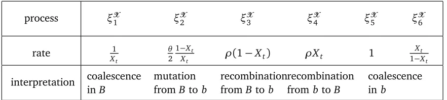
In this section we prove some key facts for the proof of Theorem 1. Recallρ=γlogαα from (3.4) and letξX1 ,ξX2 ,ξX3 ,ξX4 ,ξX5 andξX6 be Poisson-processes conditioned onX with rates X1
t,
θ
2 1−Xt
Xt ,ρ(1− Xt),ρXt, 1 and
Xt 1−Xt
, at timet, as given in Table 3. Moreover, let TiX :=supξXi be the last event of
ξXi ,i=1, ..., 4 in[0;T].
Note thatξX1 give the pair coalescence rates inB. In addition, coalescences in the wild-type back-ground might happen due to events inξX5 ∪ξX6 since 1+ Xt
1−Xt = 1
1−Xt. The other processes determine
changes in the genetic background due to mutation (ξX2 ) and recombination (ξX3 ,ξX4 ).
We will prove three Lemmata. The first deals with events of the Poisson processes during [0;T0]. Recall that T0>0 iff θ <1. The second lemma is central for (3.6), i.e., to prove that no lines are
in the beneficial background at timeT0. The third Lemma helps to order events during[T0;T]. We
process ξX1 ξX2 ξ3X ξX4 ξX5 ξ


![Table 4: Transition rates of η� in the interval [0;β0].](https://thumb-ap.123doks.com/thumbv2/123dok/971864.913932/31.612.88.516.204.267/table-transition-rates-h-interval-b.webp)