Full Terms & Conditions of access and use can be found at
http://www.tandfonline.com/action/journalInformation?journalCode=ubes20
Download by: [Universitas Maritim Raja Ali Haji] Date: 11 January 2016, At: 22:44
Journal of Business & Economic Statistics
ISSN: 0735-0015 (Print) 1537-2707 (Online) Journal homepage: http://www.tandfonline.com/loi/ubes20
Tests of Short Memory With Thick-Tailed Errors
Christine Amsler & Peter Schmidt
To cite this article: Christine Amsler & Peter Schmidt (2012) Tests of Short Memory With Thick-Tailed Errors, Journal of Business & Economic Statistics, 30:3, 381-390, DOI: 10.1080/07350015.2012.669668
To link to this article: http://dx.doi.org/10.1080/07350015.2012.669668
Accepted author version posted online: 03 Apr 2012.
Submit your article to this journal
Article views: 203
Supplementary materials for this article are available online. Please go tohttp://tandfonline.com/r/JBES
Tests of Short Memory With Thick-Tailed Errors
Christine AMSLER
Department of Economics, Michigan State University, East Lansing, MI 48824 ([email protected])
Peter SCHMIDT
Department of Economics, Michigan State University, East Lansing, MI 48824, and College of Business and Economics, Yonsei University, Seoul, Korea ([email protected])
In this article, we consider the robustness to fat tails of four stationarity tests. We also consider their sensitivity to the number of lags used in long-run variance estimation, and the power of the tests. Lo’s modified rescaled range (MR/S) test is not very robust. Choi’s Lagrange multiplier (LM) test has excellent robustness properties but is not generally as powerful as the Kwiatkowski–Phillips–Schmidt–Shin (KPSS) test. As an analytical framework for fat tails, we suggest local-to-finite variance asymptotics, based on a representation of the process as a weighted sum of a finite variance process and an infinite variance process, where the weights depend on the sample size and a constant. The sensitivity of the asymptotic distribution of a test to the weighting constant is a good indicator of its robustness to fat tails. This article has supplementary material online.
KEY WORDS: Fat tails; Robustness; Stationarity.
1. INTRODUCTION
This article considers four tests of the null hypothesis that a series is stationary and has short memory: the Kwiatkowski– Phillips–Schmidt–Shin (KPSS) test of Kwiatkowski et al. (1992), the modified rescaled range (MR/S) test of Lo (1991), the rescaled variance (V/S) test of Giraitis et al. (2003), and the Lagrange multiplier (LM, orω1) test of Choi (1994). There are a number of other tests that could have also been considered, in-cluding the tests of Leybourne and McCabe (1994,1999); Xiao (2001); Sul, Phillips, and Choi (2005); Harris, Leybourne, and McCabe (2007,2008); de Jong, Amsler, and Schmidt (2007); and Pelagatti and Sen (2009). The tests that we do consider all share the features that they depend on the cumulations of the demeaned series and they use a nonparametric long-run vari-ance estimate, so they are amenable to the same methods of asymptotic analysis.
Let the observed series beXt,t=1,. . .,T.The assumed
data-generating process under the null hypothesis is Xt =µ+εt, where εt is a zero-mean, stationary, short-memory process.
Kwiatkowski et al. (1992) and Choi (1994) considered the alter-native hypothesis to be that the series has a unit root, whereas Lo (1991) and Giraitis et al. (2003) considered the alternative to be stationary long memory. We will not distinguish these two cases carefully because tests that have power against one alternative will generally also have power against the other. For example, Lee and Schmidt (1996) and Lee and Amsler (1997) showed that the KPSS test is consistent against stationary and nonsta-tionaryI(d) alternatives. Similarly, the MR/S test and the V/S test, which are intended to have power againstI(d) alternatives, will also have power against a unit root.
In this article, we are primarily concerned with the magni-tude of possible finite sample size distortions caused by errors with thick tails. The original draft of this article (Amsler and Schmidt1999) was motivated by the intuition that these size distortions should be less for the KPSS test than for the MR/S test. Both tests depend on the cumulations of the demeaned se-ries. However, the KPSS test depends on the sum of squares of
the cumulations, while the MR/S test depends on the difference between the maximal and the minimal value of the cumulations. Intuitively, maximal and minimal values may be very sensitive to tail thickness, so that the finite sample size distortions caused by thick tails may be worse for the MR/S test than for the KPSS test. Simulations reported in that paper and in Section 3 of this article indicate that this intuition is correct. Our simulations also give some less expected results, notably that Choi’s LM test is much more robust to thick-tailed errors than the KPSS or the V/S test. This robustness comes at the expense of some sacrifice of power.
To move beyond a pure simulation study, some further an-alytical framework is needed. When the data distribution is in the domain of attraction of a stable law, different limit theories apply, based on the L´evy process. In this article, we are inter-ested in fat tailswithout infinite variance, for which standard Wiener-process asymptotics apply but may fail to be adequate in finite samples when tails are thick. We therefore consider
local-to-finite variance asymptotics, based on a representation of the seriesXtas follows:Xt =X1t+(c/g(T))X2t. Here,X1t
is a short-memory process without thick tails (e.g., normal) and
X2thas a symmetric stable distribution. The term “c” is a
con-stant, while the termg(T) is chosen so that the cumulation of
Xtconverges weakly to a weighted sum of the Wiener and L´evy
processes, with the weight depending on c. For example, for the case thatX2tis Cauchy,g(T)=
√
T. The asymptotic distri-butions of the various statistics under this representation of the process depend on the parameterc, and we evaluate the asymp-totic distributions to see which are more sensitive to the value ofc. The statistics for which the asymptotic distribution is more sensitive tocare indeed those that have more substantial size distortions with thick-tailed errors in our simulations.
© 2012American Statistical Association Journal of Business & Economic Statistics
July 2012, Vol. 30, No. 3 DOI:10.1080/07350015.2012.669668
381
2. NOTATION AND FURTHER DISCUSSION
As discussed above, let the observed series beXt,t=1,. . .,
T, whereXt=µ+εt, and whereεtis a zero-mean, stationary,
short-memory process. For the asymptotic analyses of this ar-ticle, we need to require thatεthas cumulations that satisfy a
functional central limit theorem (FCLT). For the moment, we consider the case that εt has finite variance (we will discuss
the infinite variance case later), and we assume thatεtsatisfies
the following condition (which we borrow from M¨uller2005), which therefore defines the null hypothesis.
Condition 1. (a)E(εt) = 0. (b)εt is stationary with finite
covariancesγj =E(εtεt−j). (c) σ2=∞j=−∞γj is finite and
nonzero. (d)T−1/2[rT]
t=1 εt ⇒σ W(r), where⇒indicates weak convergence, andW(r)is a Wiener process.
Define the demeaned series aset =Xt−X¯, and define the cumulation (partial sums) ofetto beSt =tj=1ej. Define the estimated autocovariances as ˆγj =T−1T
t=j+1etet−j (forj= 0, 1, 2,. . .) and define the long-run variance estimator using the Bartlett kernel andℓlags: forℓ=0,s2(ℓ) the KPSS, MR/S, and V/S statistics as follows:
KPSS=ηµˆ =T−2
Choi’s test demeans differently. Define the cumulations of the original series asCt =t
Under Condition 1, the cumulations St converge to a
mul-tiple of a Brownian bridge:T−1/2S
[rT] ⇒σ B(r) for 0≤r ≤ 1, whereB(r)=W(r)−rW(1). Then, ifs2(ℓ) is a consistent estimator of the long-run varianceσ2, the asymptotic distribu-tions of KPSS, MR/S, and V/S do not depend onσ2; they are functionals of B(r) only. This will be true if the errorsεt are
iid with mean zero and finite variance andℓis any fixed inte-ger (including zero), or it will also be true if the errors satisfy Condition 1 and the number of lags grows at an appropriate (slow) rate. Basically, we require that asT → ∞, ℓ→ ∞but ℓ/T →0. General conditions under whichs2(ℓ) is consistent can be found in de Jong and Davidson (2000) and Jansson (2002).
We will hereafter refer to the asymptotics, just discussed, as the “standard” asymptotics for these tests. They lead to 5% upper tail critical values of 0.463, 1.733, and 0.187 for the KPSS, MR/S, and V/S tests, respectively.
Similar remarks apply to Choi’s test. See Choi (1994, p. 727) for the relevant asymptotic distribution whens2(ℓ) is a consistent
estimator ofσ2. The standard asymptotics lead to a 5% upper tail critical value of approximately 0.2496 (his reported value) for Choi’s test. An interesting and, apparently, not widely under-stood feature of the standard asymptotic distribution for this test is the large amount of probability mass located near 0.25. While we were programming our simulations, we rounded 0.2496 to 0.250 and got almost no rejections. Over 8% of the probability in the asymptotic distribution turns out to lie between 0.249 and 0.250. We found (in simulations withT=10,000 and 100,000 replications) that the probability of rejection was 0.083, with a critical value of 0.249; 0.052, with a critical value of 0.2496; 0.027, with a critical value of 0.2499; and 0.002, with a critical value of 0.2500. We ultimately used a critical value of 0.249636. The point is that numerical accuracy is very, very important for this test.
In practice, Kwiatkowski et al. (1992, p. 165) recommended ℓ=o(T1/2).We will follow standard notation by defining (for integerk)ℓk=integer[k(T /100)1/4]. A popular choice for the Bartlett kernel is ℓ=ℓ12, which equals 10, 12, 14, 17, 21, 25, and 31 forT =50, 100, 200, 500, 1000, 2000, and 5000, respectively.
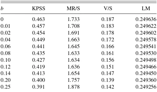
In this article, we also consider the use of critical values based on the “fixed-b” asymptotics of Kiefer and Vogelsang (2005) and Hashimzade and Vogelsang (2008). In this case, we are interested in the asymptotic distribution ofs2(ℓ), and, therefore, of the various test statistics, under the assumption thatℓ=bT, whereb∈(0,1] is a fixed constant. The point is that in finite samples, the fixed-b critical values will often lead to a better finite sample approximation to the distribution of the statistics. That is, no matter how one actually chooses the number of lags, if it is positive, the fixed-bcritical values withb=ℓ/T will give a test of more accurate size than the standard critical values, which correspond tob=0. The fixed-basymptotic distributions of the KPSS statistic, under the null that Condition 1 holds and also under the unit root alternative, are given by Amsler, Schmidt, and Vogelsang (2009), and a similar analysis would apply to the other three tests that we consider here.Table 1gives the fixed-b
upper tail 5% level critical values for the four tests considered in this article, calculated from a simulation withT =10,000 and 50,000 replications. Note that these critical values are for the case that the Bartlett kernel is used; different kernels lead to different fixed-bcritical values.
Table 1. Fixed-b5% upper tail critical values for the four tests using Bartlett kernel
Amsler and Schmidt: Tests of Short Memory With Thick-Tailed Errors 383
3. SIMULATIONS
In this section, we report the results of simulations de-signed to compare the finite sample size and the power of our four tests. The data-generating process is very simple: theXt, t=1, . . . , T ,are iid. The data are centered on zero (µ=0). We consider sample sizes T =50, 100, 200, 500, 1000, and 2000. The following distributions forXt are considered:
stan-dard normal; Student’stwith 10, 5, 3, and 2 degrees of freedom; and standard Cauchy. All the four tests are valid asymptotically for the normal case and for thet-distributions with 10, 5, or 3 degrees of freedom. The standard and fixed-basymptotics are not valid for the Cauchy case, for which the mean does not exist and the variance is infinite. The case of thet2 distribution is more interesting. This distribution has an infinite variance but its variance is “just barely infinite” in the sense of Kourogenis and Pittis (2008) (it has finite absolute moments of orderδfor δ <2). Abadir and Magnus (2004) showed that thet2 distribu-tion is in the domain of attracdistribu-tion, but not in the normal domain of attraction, of a normal distribution. Specifically, it follows a central limit theorem but with a nonstandard normalization of (T ·lnT)−1/2. The results by Kourogenis and Pittis also apply, and so, an invariance principle holds. As a result, it is reasonable to presume that all of the tests we consider will be asymptoti-cally valid in this case. However, a proof of that result would be a detour from the path of this article and we will not pursue it.
We have attempted to pick distributions forXtthat span the
empirically relevant range. Few studies report the kurtosis of the data so that is a bit hard to know. One simple example, in de Jong, Amsler, and Schmidt (2007, p. 321), reported kurtoses ranging from 4.84 to 11.05 for five nominal exchange rate series. Since the kurtosis for at-distribution withkdegrees of freedom is 3+ 6/(k– 4), these kurtoses are consistent witht-distributions with
kin the range of 5–7, that is, with moderately fat tails.
The data are generated by drawing pseudo-random normal deviates and transforming them as appropriate. (For example, the Cauchy is the ratio of two standard normals.) The number of replications was 25,000 forT=1000 and 2000, and 50,000 for the other sample sizes. We consider only upper tail 5% tests. We consider the case ofℓ=0 and alsoℓ=ℓ12 (whereℓk= integer[k(T /100)1/4]). The use ofℓ >0 is unnecessary with iid data, but was considered because we want to see how sensitive the various tests are to the choice ofℓ.
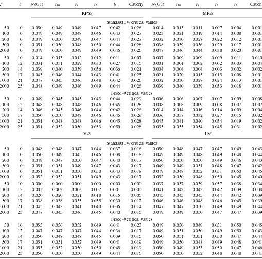
Table 2gives the size of the various tests, using the standard and the fixed-bcritical values. There is an expanded version of this table in the online Appendix to this article. We will discuss first the case thatℓ=0, in which case there is no distinction between these two sets of critical values.
For the cases where the standard asymptotics apply (normal, andt-distribution with three or more degrees of freedom), the KPSS, V/S, and LM tests are all quite accurate (have size close to 0.05) for all sample sizes, evenT=50. This is not true for the MR/S test, however. For example, note its size, in the normal case, of 0.014, 0.023, 0.032, and 0.038 forT=50, 100, 200, and 500, respectively. Apparently, its convergence to its asymptotic distribution is slower than that for the other three tests.
Next, consider the issue of robustness to fat tails. Here, there is a very clear ranking: the LM test is the best, and the MR/S test is the worst. The KPSS test is marginally better than the V/S
test. For example, note the size forT=2000 in the Cauchy case: 0.026, 0.001, 0.017, and 0.042 for the KPSS, MR/S, V/S, and LM tests, respectively. The MR/S test essentially does not reject in the Cauchy case. These results are similar for smaller sample sizes as well. A very general conclusion from these results is that, except for the MR/S test, fat tails are not really a serious problem. It takes a very extreme distribution, such as Cauchy, before the size distortions are large enough to be worrisome.
Now consider the case that ℓ12 lags are used. When the standard critical levels are used, more lags cause size distortions (too few rejections). The LM test is only minimally affected by the number of lags, but for the other tests, these size distortions can be large. For example, withT=200 andℓ12 (=14) lags, size in the normal case is 0.039, 0.004, 0.020, and 0.045 for the KPSS, MR/S, V/S, and LM tests. The size distortions caused by a large number of lags are more or less completely eliminated (except for the MR/S test at the smaller sample sizes) by using the fixed-b critical values. This basically is the argument for using the fixed-bcritical values.
Amsler and Schmidt (2012) considered the robustness of the four tests considered here to autocorrelation, namely first-order autoregressive [AR(1)] errors with parameters 0.8 and 0.9. Their results showed that the LM test is far more robust to autocorre-lation than the other three tests. So, in terms of robustness to fat tails, to the number of lags used, and to short-run dynamics, the LM test appears to be the best of the four tests.
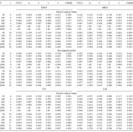
Table 3 gives the power of the tests against a unit root al-ternative. The online Appendix contains an expanded version of this table. The parameterization of the alternative is a slight generalization of the data-generating process (DGP) in KPSS, to accommodate cases of infinite variance. We generate the series asXt =λ1/2rt+εt,rt =rt−1+ut, where theεanduprocesses are iid and both are drawn from the same distribution (normal,t, or Cauchy). The null hypothesis isλ=0 and we give results for the alternative thatλ=0.01. Amsler and Schmidt gave results for some other values ofλ,for KPSS and MR/S only, but the results forλ=0.01 are representative. We considerT=50, 100, 200, 500, 1000, and 2000, as above, andℓ=0 andℓ=ℓ12.
Consider first the results for ℓ=0, for which the fixed-b
critical values are the same as the standard critical values. The most striking result is that the LM test is less powerful than the other three tests. There is a tendency for the KPSS test to have a higher power than the V/S test when power is low, and vice versa, but the similarities outweigh the differences. The power of the MR/S test is generally low, but it is not low in those cases in which it did not suffer from large size distortions under the null.
The conclusions for the case that ℓ=ℓ12 and we use the size-adjusted critical values are very similar.
We also consider size-adjusted power. Apart from the Cauchy case, the size distortions when fixed-b critical values are used were small for all of the tests except the MR/S test. So, to save space, we give size-adjusted power only for the KPSS and MR/S tests. The results for the other two distributions are provided in the online Appendix. There are some anomalous results for cases with smallTand largeℓ, but the power of the MR/S test is now comparable with or often even slightly larger than the power of the KPSS test. Apparently, its problem is not an intrinsic lack of power, but just poor size control.
Table 2. Size of various tests
T ℓ N(0,1) t10 t5 t3 t2 Cauchy N(0,1) t10 t5 t3 t2 Cauchy
KPSS MR/S
Standard 5% critical values
50 0 0.050 0.049 0.049 0.047 0.042 0.026 0.014 0.013 0.011 0.007 0.004 0.001
100 0 0.049 0.049 0.048 0.046 0.043 0.027 0.023 0.021 0.019 0.014 0.008 0.001
200 0 0.049 0.050 0.049 0.047 0.044 0.027 0.032 0.030 0.028 0.022 0.012 0.001
500 0 0.051 0.050 0.048 0.050 0.044 0.028 0.038 0.039 0.036 0.029 0.017 0.001
2000 0 0.049 0.050 0.049 0.049 0.046 0.026 0.047 0.046 0.044 0.038 0.020 0.001
50 10 0.014 0.013 0.012 0.012 0.011 0.007 0.007 0.009 0.009 0.009 0.011 0.010
100 12 0.031 0.031 0.029 0.030 0.027 0.015 0.001 0.001 0.002 0.002 0.003 0.004
200 14 0.039 0.040 0.039 0.036 0.036 0.021 0.004 0.004 0.004 0.003 0.002 0.002
500 17 0.045 0.046 0.044 0.043 0.041 0.025 0.021 0.020 0.015 0.015 0.008 0.001
1000 21 0.047 0.045 0.046 0.048 0.042 0.026 0.032 0.030 0.028 0.024 0.013 0.001
2000 25 0.048 0.049 0.046 0.049 0.044 0.026 0.039 0.040 0.039 0.033 0.018 0.001
Fixed-bcritical values
50 10 0.049 0.045 0.045 0.043 0.044 0.029 0.006 0.006 0.007 0.007 0.009 0.008
100 12 0.048 0.048 0.048 0.046 0.045 0.028 0.008 0.008 0.009 0.008 0.007 0.007
200 14 0.046 0.045 0.046 0.044 0.042 0.026 0.014 0.014 0.016 0.014 0.009 0.004
500 17 0.050 0.050 0.048 0.046 0.045 0.029 0.036 0.037 0.032 0.027 0.015 0.002
1000 21 0.051 0.048 0.048 0.046 0.045 0.028 0.043 0.041 0.040 0.034 0.019 0.002
2000 25 0.051 0.052 0.050 0.053 0.050 0.028 0.055 0.055 0.054 0.045 0.031 0.002
V/S LM
Standard 5% critical values
50 0 0.048 0.048 0.047 0.044 0.037 0.016 0.050 0.048 0.047 0.047 0.049 0.043
100 0 0.050 0.049 0.045 0.046 0.038 0.018 0.049 0.049 0.048 0.049 0.048 0.044
200 0 0.049 0.047 0.050 0.047 0.040 0.017 0.050 0.050 0.050 0.049 0.046 0.043
500 0 0.051 0.051 0.049 0.047 0.043 0.017 0.049 0.049 0.051 0.048 0.047 0.042
1000 0 0.051 0.051 0.050 0.050 0.043 0.018 0.049 0.048 0.052 0.051 0.050 0.045
2000 0 0.052 0.052 0.051 0.049 0.043 0.017 0.052 0.050 0.048 0.050 0.045 0.040
50 10 0.000 0.000 0.000 0.000 0.000 0.000 0.037 0.037 0.039 0.037 0.038 0.034
100 12 0.003 0.002 0.003 0.002 0.001 0.000 0.041 0.042 0.042 0.042 0.039 0.038
200 14 0.020 0.020 0.021 0.018 0.015 0.005 0.045 0.045 0.045 0.044 0.042 0.039
500 17 0.038 0.038 0.035 0.035 0.030 0.012 0.046 0.046 0.048 0.046 0.045 0.039
1000 21 0.045 0.042 0.041 0.040 0.036 0.014 0.047 0.047 0.050 0.049 0.049 0.044
2000 25 0.047 0.045 0.046 0.045 0.040 0.015 0.049 0.049 0.050 0.047 0.047 0.039
Fixed-bcritical values
50 10 0.055 0.056 0.052 0.049 0.041 0.023 0.049 0.050 0.049 0.051 0.050 0.045
100 12 0.047 0.047 0.047 0.044 0.036 0.017 0.049 0.051 0.050 0.049 0.050 0.043
200 14 0.050 0.048 0.048 0.045 0.039 0.016 0.050 0.051 0.051 0.050 0.047 0.044
500 17 0.051 0.051 0.052 0.049 0.041 0.019 0.049 0.050 0.048 0.049 0.048 0.041
1000 21 0.053 0.052 0.050 0.050 0.045 0.019 0.050 0.049 0.053 0.050 0.047 0.046
2000 25 0.050 0.050 0.050 0.049 0.044 0.016 0.050 0.050 0.052 0.048 0.048 0.041
4. LOCAL-TO-FINITE VARIANCE ASYMPTOTICS
We continue to assume the modelXt =µ+εt. However, we now consider cases whereεtmay have infinite variance, which is
a violation of Condition 1. We make the following assumption.
Condition 2. (a)εtisiid. (b)εtis distributed symmetrically
around zero. (c) εt is in the normal domain of attraction of a
stable law with indexα, with 0< α <2.
Define [UT(r), VT(r)]=[T−1/α[rT]
j=1εj, T−2/α [rT]
j=1ε 2
j]. Then, Chan and Tran (1989) showed the following result: if Condition 2 holds, [UT(r), VT(r)]⇒[Uα(r), Vα(r)].
Here, Uα(r) is a standard stable process (L´evy process), with indexαandVα(r)=0r(dUα(s))
2ds
. See Phillips (1990,
p. 46) for further discussion and definitions of terms. See also Ahn, Fotopoulos, and He (2001) for a good expository treatment of these results and their application to unit root tests.
This result is easily extended to the demeaned data. Let X∗
t =Xt−X¯ =εt−ε¯ ≡εt∗, let UT∗(r) andVT∗(r) be defined in the same way asUT(r) andVT(r), except withXj∗ (or ε∗j) replacingεj, and letUα∗(r)=Uα(r)−rUα(1), the analog of a Brownian bridge, andV∗
α(r)=
r
0 (dUα∗(s))2ds. Then, the same convergence result that was given above forUT(r) andVT(r) still holds, with these replacements (i.e.,U∗
T(r) in place ofUT(r), U∗
α(r) in place ofUα(r), etc.); see Phillips (1990, p. 55). Amsler and Schmidt (1999) used these results to prove the following result.
Amsler and Schmidt: Tests of Short Memory With Thick-Tailed Errors 385
Table 3. Power of various tests,λ=0.01
T ℓ N(0,1) t10 t5 t3 t2 Cauchy N(0,1) t10 t5 t3 t2 Cauchy
KPSS MR/S
Fixed-bcritical values
50 0 0.293 0.294 0.300 0.307 0.327 0.396 0.126 0.125 0.129 0.138 0.167 0.275
100 0 0.593 0.591 0.583 0.588 0.587 0.566 0.517 0.512 0.506 0.504 0.495 0.482
200 0 0.848 0.851 0.848 0.846 0.822 0.727 0.875 0.874 0.874 0.860 0.815 0.679
500 0 0.988 0.988 0.987 0.986 0.973 0.873 0.997 0.997 0.996 0.995 0.979 0.852
1000 0 1.00 1.00 1.00 1.00 0.996 0.924 1.00 1.00 1.00 1.00 0.997 0.924
2000 0 1.00 1.00 1.00 1.00 0.999 0.966 1.00 1.00 1.00 1.00 0.999 0.961
50 10 0.194 0.190 0.197 0.199 0.208 0.165 0.002 0.002 0.003 0.003 0.004 0.009
100 12 0.430 0.432 0.423 0.428 0.430 0.428 0.004 0.003 0.003 0.004 0.005 0.005
200 14 0.640 0.642 0.640 0.646 0.641 0.598 0.284 0.282 0.277 0.273 0.274 0.289
500 17 0.868 0.868 0.870 0.873 0.866 0.745 0.885 0.883 0.882 0.886 0.870 0.738
1000 21 0.953 0.954 0.954 0.955 0.949 0.896 0.974 0.975 0.976 0.972 0.969 0.883
2000 25 0.988 0.988 0.989 0.989 0.989 0.954 0.997 0.998 0.998 0.998 0.997 0.953
Size-adjusted power
50 0 0.296 0.295 0.301 0.316 0.344 0.426 0.242 0.246 0.255 0.330 0.334 0.441
100 0 0.546 0.593 0.596 0.596 0.603 0.598 0.597 0.598 0.606 0.618 0.628 0.617
200 0 0.851 0.851 0.848 0.850 0.831 0.752 0.891 0.896 0.895 0.896 0.875 0.771
500 0 0.987 0.988 0.987 0.986 0.975 0.886 0.997 0.997 0.997 0.996 0.985 0.899
1000 0 1.00 0.999 1.00 1.00 0.996 0.941 1.00 1.00 1.00 1.00 0.999 0.947
2000 0 1.00 1.00 1.00 1.00 1.00 0.970 1.00 1.00 1.00 1.00 1.00 0.974
50 10 0.198 0.202 0.207 0.217 0.231 0.301 0.025 0.025 0.026 0.027 0.027 0.029
100 12 0.434 0.433 0.428 0.433 0.444 0.472 0.032 0.036 0.034 0.042 0.054 0.185
200 14 0.649 0.647 0.648 0.660 0.652 0.636 0.477 0.486 0.499 0.515 0.555 0.601
500 17 0.870 0.868 0.872 0.879 0.872 0.824 0.900 0.899 0.905 0.913 0.919 0.857
1000 21 0.955 0.955 0.956 0.954 0.955 0.910 0.977 0.977 0.979 0.981 0.982 0.933
2000 25 0.988 0.988 0.989 0.989 0.990 0.959 0.997 0.998 0.997 0.998 0.998 0.969
V/S LM
Fixed-bcritical values
50 0 0.241 0.243 0.250 0.262 0.285 0.361 0.073 0.073 0.078 0.089 0.117 0.219
100 0 0.598 0.592 0.592 0.593 0.585 0.553 0.296 0.295 0.295 0.302 0.322 0.382
200 0 0.887 0.887 0.884 0.880 0.848 0.723 0.586 0.586 0.582 0.583 0.583 0.553
500 0 0.995 0.996 0.995 0.995 0.982 0.877 0.814 0.814 0.816 0.814 0.808 0.734
1000 0 1.00 1.00 1.00 1.00 0.997 0.937 0.897 0.898 0.900 0.898 0.892 0.831
2000 0 1.00 1.00 1.00 1.00 0.999 0.967 0.940 0.940 0.939 0.939 0.938 0.892
50 10 0.059 0.060 0.057 0.057 0.050 0.033 0.030 0.031 0.029 0.030 0.030 0.028
100 12 0.305 0.301 0.303 0.300 0.299 0.287 0.020 0.020 0.021 0.021 0.019 0.022
200 14 0.677 0.676 0.679 0.671 0.655 0.565 0.070 0.070 0.070 0.067 0.065 0.054
500 17 0.920 0.919 0.919 0.922 0.910 0.809 0.524 0.521 0.521 0.527 0.524 0.492
1000 21 0.983 0.984 0.983 0.981 0.975 0.907 0.667 0.664 0.672 0.671 0.676 0.659
2000 25 0.998 0.998 0.997 0.998 0.997 0.956 0.760 0.758 0.762 0.760 0.766 0.762
Proposition 1. Suppose thatXt =µ+εtand thatεtsatisfies
Condition 2. Then,
ˆ ηµ(0)⇒
1
0
Uα∗(r)2dr/Vα∗(1). (5)
The only interesting technical detail is the way the normalization of the sums is implicitly handled:
ˆ
ηµ(0) = T−2
tS
2
t / T−
1
t (X∗t)
2
= T−1
t(T−
1/αSt)2/
T−2/α
t(X∗t)
2. That is, the partial sums of the data converge
at a different rate in the infinite variance case than in the finite variance case, but the statistic converges at the same rate.
Phillips (1990, p. 50) showed how to modify these results to allow certain forms of short-run dependence. Specifically, he al-lowed for a linear process:εt =d(L)ut =∞
j=0djut−j, where
utsatisfiesCondition 2and 0<d(1)<∞. Under this
assump-tion, he showed that the semiparametric correction designed for the finite variance case works also in the infinite variance case. Neither the infinite variance asymptotics nor the finite vari-ance asymptotics may do a good job of approximating the distri-bution of the stationarity test statistics when the data have a finite variance but fat tails. Basically, we want to find a way to move continuously from the normal case to the Cauchy case, and the
t-distributions with varying degrees of freedom (which we used in our earlier simulations) did not accomplish this. We therefore
consider alocal-to-finite varianceparameterization that may be able to do so. This is based on the following representation of the seriesεt:
εt =ε1t+
c/T[(1/α)−(1/2)]ε2t, (6)
whereε1tsatisfies Condition 1 (has finite variance) andε2t
sat-isfies Condition 2 (has infinite variance). Here,cis an arbitrary constant that weights the two components ofεt. The order in
probability of the cumulations of the infinite variance process ε2tis larger than that of the cumulations of the finite variance
processε1t, and the power ofTin the representation (6) is
cho-sen so that the cumulation of the seriesεt, suitably normalized,
converges to a stochastic process that is the weighted sum of a Wiener process and a L´evy process.
We call this a local-to-finite variance representation because εt has infinite variance for allT, but loosely speaking, it
con-verges to a finite variance process as T → ∞. This is philo-sophically similar to other types of local representations, such as local to an autoregressive unit root (e.g., Elliott, Rothenberg, and Stock1996) or local to a unit moving average root (Pantula 1991) or local to useless instruments (Staiger and Stock1997), in that it is an attempt to create asymptotics that can be used to analyze features of the data that are relevant in finite samples but not in the standard asymptotics.
The situation in the literature on the local-to-finite variance parameterization and related convergence results is somewhat unusual. The parameterization was first suggested and the proofs of the asymptotic results given in the current article were pre-sented by Amsler and Schmidt (1999), but that paper was never published. These results were used, and some of them were proved again, by Callegari, Cappuccio, and Lubian (2003) and Cappuccio and Lubian (2007). Those articles quoted Amsler and Schmidt (1999) but gave a somewhat self-contained pre-sentation of the results. In the current article, we will simply quote these results and indicate how we use them.
The basic convergence result is the following.
Proposition 2. Suppose thatεtsatisfiesEquation (6), where
ε1tsatisfies Condition 1 andε2tsatisfies Condition 2. Then,
T−1/2
To allow for the fact that the data for the KPSS, MR/S, and V/S tests are in deviations from means, we introduce the analog of a Brownian bridge: G∗
α,c(r)=Gα,c(r)−rGα,c(1). Amsler and Schmidt (1999) derived the asymptotic distribution of the KPSS statistic with no lags (ℓ=0), which is exactly as in Equa-tion (5)except thatG∗α,c(r) replacesUα∗(r) in the numerator of the expression for the asymptotic distribution. That is,
ˆ
Cappuccio and Lubian (2007) also derived these results for the KPSS and MR/S tests, as well as the LM test and several other tests. We will therefore omit the proofs here.
We note that the same asymptotic distribution holds if the number of lags is positive and grows at an appropriate rate. A
precisely stated proposition and its proof are given in the online Appendix.
5. SIMULATIONS WITH LOCAL-TO-FINITE VARIANCE DATA
We now return to the question of the relative robustness of the KPSS, MR/S, V/S, and LM tests to thick tails. We use the local-to-finite variance asymptotics in a conceptually simple way. The asymptotic distribution of each of the statistics depends on the quantity “c” that determines the relative weight of the infinite variance component. We will say that one statistic is more robust than another if its asymptotic distribution is less sensitive to the value ofc.
Before we make such comparisons, we first present the results of some simulations that investigate the finite sample accuracy of the local-to-finite variance asymptotics. In these simulations, we consider only the statistics withℓ=0, and we consider the case thatε1t is standard normal whileε2t is Cauchy (α=1).
Therefore,εt =ε1t+(c/
√
T)ε2t. We considerT between 50 and 2000, as before, and c=0, 0.1, 0.316, 1, 3.16, 10, and 31.6. (Here, 3.16 is shorthand for√10, etc.) Values ofclarger than 31.6 had only very minimal effects on the results; we have essentially reached the pure Cauchy case. The number of replications is 50,000 except that it is only 25,000 forT=1000 or 2000. These simulations are similar to those of Cappuccio and Lubian (2007,Table 2), who considered more values ofα but less values ofT.
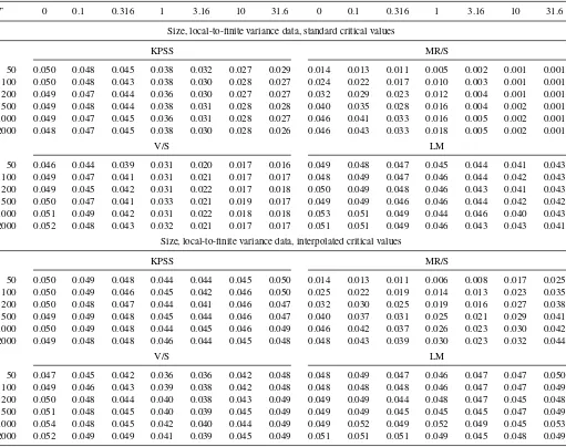
The results of these simulations are given in the top half of Table 4, where we report the size (frequency of rejection) of the 5% upper tail tests. For the KPSS, V/S, and LM tests, the asymptotics are quite reliable, in the sense that, holdingc
constant, changingT did not have much effect on the results. For the MR/S test, the asymptotics are not very reliable forT≤
200, but they seemed fairly reliable forT≥500. Reading across the table horizontally, we can observe a smooth increase in the size distortions of all of the tests as we move from the normal case (c=0) to the near Cauchy case (c=31.6). As inTable 2, we can observe that the size distortions are biggest for the MR/S test and smallest for the LM test.
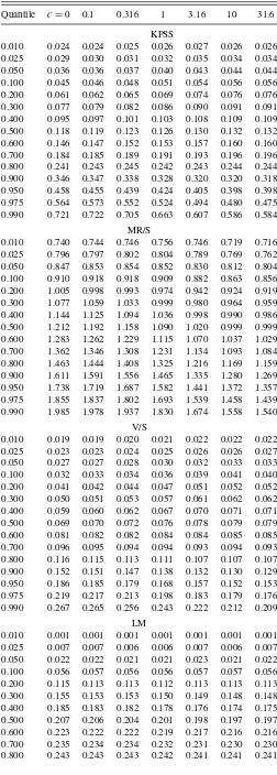
We now return to the task of assessing the relative sensitivity of the asymptotic distributions of the various test statistics to the value ofc. We have evaluated the distributions of the statistics by simulation forT=10,000, using 100,000 replications. Various quantiles are presented inTable 5. There is a question of how to measure the sensitivity of these distributions to the value of
c. Rather than use a summary statistic, we simply provide all of the deciles of the distributions, as well as the 0.001, 0.025, 0.050, 0.950, 0.975, and 0.999 quantiles.
For the LM statistic, there are only minor changes in any of the quantiles ascchanges. Thus, the LM test is very robust to fat tails, as we saw in Section 3.
For the KPSS statistic, the shifts in the asymptotic distribution ascchanges are relatively minor. Most of the distribution shifts slightlyrightascincreases. For example, the median is 0.118 for
c=0 and rises to 0.132 forc=31.6. Most of the other quantiles show a similar pattern. However, the upper tail quantiles are the exception; theydecreaseascincreases. For example, the 0.950 quantile decreases from 0.476 to 0.395 ascincreases from 0 to
Amsler and Schmidt: Tests of Short Memory With Thick-Tailed Errors 387
Table 4. Size (frequency of rejection) of the 5% upper tail tests
T 0 0.1 0.316 1 3.16 10 31.6 0 0.1 0.316 1 3.16 10 31.6
Size, local-to-finite variance data, standard critical values
KPSS MR/S
50 0.050 0.048 0.045 0.038 0.032 0.027 0.029 0.014 0.013 0.011 0.005 0.002 0.001 0.001
100 0.050 0.048 0.043 0.038 0.030 0.028 0.027 0.024 0.022 0.017 0.010 0.003 0.001 0.001
200 0.049 0.047 0.044 0.036 0.030 0.027 0.027 0.032 0.029 0.023 0.012 0.004 0.001 0.001
500 0.049 0.048 0.044 0.038 0.031 0.028 0.028 0.040 0.035 0.028 0.016 0.004 0.002 0.001
1000 0.049 0.047 0.045 0.036 0.031 0.028 0.027 0.046 0.041 0.033 0.016 0.005 0.002 0.001
2000 0.048 0.047 0.045 0.038 0.030 0.028 0.026 0.046 0.043 0.033 0.018 0.005 0.002 0.001
V/S LM
50 0.046 0.044 0.039 0.031 0.020 0.017 0.016 0.049 0.048 0.047 0.045 0.044 0.041 0.043
100 0.049 0.047 0.041 0.031 0.021 0.017 0.017 0.048 0.049 0.047 0.046 0.044 0.042 0.043
200 0.049 0.045 0.042 0.031 0.022 0.017 0.018 0.050 0.049 0.048 0.046 0.043 0.041 0.043
500 0.050 0.047 0.041 0.033 0.021 0.019 0.017 0.049 0.049 0.046 0.046 0.044 0.042 0.042
1000 0.051 0.049 0.042 0.031 0.022 0.018 0.018 0.053 0.051 0.049 0.044 0.046 0.040 0.043
2000 0.052 0.048 0.043 0.032 0.021 0.017 0.017 0.051 0.051 0.049 0.046 0.043 0.043 0.041
Size, local-to-finite variance data, interpolated critical values
KPSS MR/S
50 0.050 0.049 0.048 0.044 0.044 0.045 0.050 0.014 0.013 0.011 0.006 0.008 0.017 0.025
100 0.050 0.049 0.046 0.045 0.042 0.046 0.050 0.025 0.022 0.019 0.014 0.013 0.023 0.035
200 0.050 0.048 0.047 0.044 0.041 0.046 0.047 0.032 0.030 0.025 0.019 0.016 0.027 0.038
500 0.049 0.049 0.048 0.045 0.044 0.046 0.047 0.040 0.037 0.031 0.025 0.021 0.029 0.041
1000 0.050 0.049 0.048 0.044 0.045 0.046 0.049 0.046 0.042 0.037 0.026 0.023 0.030 0.042
2000 0.049 0.048 0.048 0.046 0.044 0.045 0.048 0.048 0.043 0.039 0.030 0.023 0.032 0.044
V/S LM
50 0.047 0.045 0.042 0.036 0.036 0.042 0.048 0.048 0.049 0.047 0.046 0.047 0.047 0.050
100 0.049 0.046 0.043 0.039 0.038 0.042 0.048 0.048 0.048 0.048 0.046 0.047 0.047 0.049
200 0.050 0.048 0.044 0.040 0.038 0.043 0.049 0.049 0.049 0.044 0.048 0.047 0.045 0.048
500 0.051 0.048 0.045 0.040 0.039 0.045 0.049 0.049 0.049 0.045 0.045 0.045 0.047 0.049
1000 0.054 0.048 0.045 0.042 0.040 0.044 0.049 0.049 0.052 0.049 0.052 0.049 0.045 0.053
2000 0.052 0.049 0.049 0.041 0.039 0.045 0.049 0.051 0.051 0.051 0.049 0.045 0.048 0.049
31.6. This explains the smaller number of rejections of the null whencincreases, since we are using an upper tail test.
For the V/S statistic, the pattern is quite similar to that for KPSS. However, the changes are bigger for V/S than for KPSS, and indeed, in Section 3, we saw that the V/S test was less robust to fat tails than the KPSS test.
For the MR/S statistic, things are rather different. The asymp-totic distribution shifts left ascincreases, and this is true across the whole distribution. The shift is largest in the upper tail. For example, as we move fromc=0 toc=31.6, the median changes from 1.216 to 0.999, while the 0.95 quantile changes from 1.739 to 1.361. These changes are larger for the MR/S statistic than for the KPSS statistic, for example, and this at least partially explains the lower degree of robustness of the MR/S test to fat tails. However, the thickness of the tails of the distributions of the test statistics under thick-tailed errors is also relevant. For example, the change in the 0.95 quantile as we go from normal to Cauchy errors is larger but not terribly larger in percentage terms for the MR/S statistic compared with the KPSS statistic (1.739 becomes 1.361 for MR/S, while 0.476 becomes 0.395 for KPSS). But the implication of this change for rejections
un-der the null is very different, because the longer tail of KPSS (compared with MR/S) in the Cauchy case puts a much higher fraction of observations above the standard critical value.
An interesting question is whether the size distortions that arise whencis nonzero can be reduced by estimatingcand then using the appropriate critical value based on the estimated value ofc.Obviously, in some sense, this must depend on how well one can estimatec. To be more explicit, letεt=ε1t+(c/
√
T)ε2tas discussed above, and defineγ =c/√T. As we will show, it is possible to find a√T-consistent estimate ofγ, say ˆγ, so that
ˆ
γ −γ =Op(T−1/2). Then, we define ˆc
=√Tγˆso that ˆc−c= Op(1). That is, we can estimatecthough not consistently. As a practical matter, this does not indicate whether or not we can estimate it reasonably well; it just implies that any corrections to the critical values based on the estimatedcwill not necessarily improve as the sample size increases.
To be more precise, we observe deviations from means of [σ · N(0,1) + γ·Cauchy], and we need to estimate the two parametersσ andγ, and then calculate ˆc=√T( ˆγ /σˆ). (Divi-sion by an estimate ofσis necessary because the discussion of the local-to-finite variance parameterization above hadσ =1,
Table 5. Quantiles of test statistics, local-to-finite variance data
Quantile c=0 0.1 0.316 1 3.16 10 31.6
KPSS
0.010 0.024 0.024 0.025 0.026 0.027 0.026 0.026
0.025 0.029 0.030 0.031 0.032 0.035 0.034 0.034
0.050 0.036 0.036 0.037 0.040 0.043 0.044 0.044
0.100 0.045 0.046 0.048 0.051 0.054 0.056 0.056
0.200 0.061 0.062 0.065 0.069 0.074 0.076 0.076
0.300 0.077 0.079 0.082 0.086 0.090 0.091 0.091
0.400 0.095 0.097 0.101 0.103 0.108 0.109 0.109
0.500 0.118 0.119 0.123 0.126 0.130 0.132 0.132
0.600 0.146 0.147 0.152 0.153 0.157 0.160 0.160
0.700 0.184 0.185 0.189 0.191 0.193 0.196 0.196
0.800 0.241 0.243 0.245 0.242 0.243 0.244 0.244
0.900 0.346 0.347 0.338 0.328 0.320 0.320 0.318
0.950 0.458 0.455 0.439 0.424 0.405 0.398 0.398
0.975 0.564 0.573 0.552 0.524 0.494 0.480 0.475
0.990 0.721 0.722 0.705 0.663 0.607 0.586 0.584
MR/S
0.010 0.740 0.744 0.746 0.756 0.746 0.719 0.716
0.025 0.796 0.797 0.802 0.804 0.789 0.769 0.762
0.050 0.847 0.853 0.854 0.852 0.830 0.812 0.804
0.100 0.910 0.918 0.918 0.909 0.882 0.863 0.856
0.200 1.005 0.998 0.993 0.974 0.942 0.924 0.919
0.300 1.077 1.059 1.033 0.999 0.980 0.964 0.959
0.400 1.144 1.125 1.094 1.036 0.998 0.990 0.986
0.500 1.212 1.192 1.158 1.090 1.020 0.999 0.999
0.600 1.283 1.262 1.229 1.115 1.070 1.037 1.029
0.700 1.362 1.346 1.308 1.231 1.134 1.093 1.084
0.800 1.463 1.444 1.408 1.325 1.216 1.169 1.159
0.900 1.611 1.591 1.556 1.465 1.335 1.280 1.269
0.950 1.738 1.719 1.687 1.582 1.441 1.372 1.357
0.975 1.855 1.837 1.802 1.693 1.539 1.458 1.439
0.990 1.985 1.978 1.937 1.830 1.674 1.558 1.540
V/S
0.010 0.019 0.019 0.020 0.021 0.022 0.022 0.022
0.025 0.023 0.023 0.024 0.025 0.026 0.026 0.027
0.050 0.027 0.027 0.028 0.030 0.032 0.033 0.033
0.100 0.032 0.033 0.034 0.036 0.039 0.041 0.040
0.200 0.041 0.042 0.044 0.047 0.051 0.052 0.052
0.300 0.050 0.051 0.053 0.057 0.061 0.062 0.062
0.400 0.059 0.060 0.062 0.067 0.070 0.071 0.071
0.500 0.069 0.070 0.072 0.076 0.078 0.079 0.079
0.600 0.081 0.082 0.082 0.084 0.084 0.085 0.085
0.700 0.096 0.095 0.094 0.094 0.093 0.094 0.093
0.800 0.116 0.115 0.113 0.111 0.107 0.107 0.107
0.900 0.152 0.151 0.147 0.138 0.132 0.130 0.129
0.950 0.186 0.185 0.179 0.168 0.157 0.152 0.153
0.975 0.219 0.217 0.213 0.198 0.183 0.179 0.176
0.990 0.267 0.265 0.256 0.243 0.222 0.212 0.209
LM
0.010 0.001 0.001 0.001 0.001 0.001 0.001 0.001
0.025 0.007 0.007 0.006 0.006 0.007 0.006 0.007
0.050 0.022 0.022 0.021 0.021 0.023 0.021 0.022
0.100 0.056 0.057 0.056 0.056 0.057 0.057 0.056
0.200 0.115 0.113 0.113 0.112 0.113 0.113 0.113
0.300 0.155 0.153 0.153 0.150 0.149 0.148 0.148
0.400 0.185 0.183 0.182 0.178 0.176 0.174 0.175
0.500 0.207 0.206 0.204 0.201 0.198 0.197 0.197
0.600 0.223 0.222 0.222 0.219 0.217 0.216 0.216
0.700 0.235 0.234 0.234 0.232 0.231 0.230 0.230
0.800 0.243 0.243 0.243 0.242 0.241 0.241 0.241
Table 5. (continued)Quantiles of test statistics, local-to-finite variance data
Quantile c=0 0.1 0.316 1 3.16 10 31.6
0.900 0.248 0.248 0.248 0.248 0.247 0.248 0.247
0.950 ∗628 ∗656 ∗563 ∗610 ∗556 ∗489 ∗477
0.975 ∗911 ∗916 ∗900 ∗914 ∗892 ∗863 ∗877
0.990 ∗990 ∗988 ∗986 ∗989 ∗984 ∗980 ∗981
NOTE:∗628 means 0.249628,∗656 means 0.249656, etc.
which is empirically restrictive.) We will use a very simple con-sistent estimator ofσandγobtained by matching the empirical and theoretical characteristic functions of the deviations from means ofεtfor two values (0.2 and 1.0) of its argument. Details
are given in the Appendix. We then find critical values for the various tests, for the estimated value ofc, by interpolating in Table 5in the rows corresponding to the 0.95 quantiles.
The results are given in the bottom half ofTable 4. The inter-polation procedure works reasonably (and perhaps surprisingly) well. For all of the tests, the size distortions when the interpo-lated critical values are used are considerably smaller than when the standard critical values are used. Of course, this is most true whencis large, because that is when the size distortions were biggest to begin with. Interestingly, we do not estimatecas well when it is large as when it is small, but whenc is large, the critical values are much less sensitive to its value than when it is small.
6. CONCLUDING REMARKS
In this article, we have considered four tests of the null hy-pothesis that a series is stationary and has short memory. We are primarily interested in their robustness to fat tails. A very general conclusion from our simulations is that, except for the MR/S test, fat tails are not really a very serious problem. It takes a very extreme distribution, such as Cauchy, before the size distortions are large enough to be worrisome.
However, there were nontrivial differences between the var-ious tests. The LM test was by far the most robust to fat tails. This was true in our basic simulations, and it was also evident in our analysis of the local-to-finite variance asymptotic distri-butions. It was true in the case of no lags (ℓ=0) and also when a large number of lags were used. [The LM test is also by far the most robust to error autocorrelation, as reported by Amsler and Schmidt (2012).] So, it had excellent size properties. Unfor-tunately, it was the least powerful of the four tests against unit root alternatives. Perhaps unsurprisingly, excellent size control comes at some price in power.
At the other extreme, Lo’s MR/S test was very nonrobust to small sample sizes (it was slow to converge to its asymptotic distribution) and also to fat tails. It was often substantially un-dersized and this carried over into low apparent power against unit root alternatives. However, it did reasonably well in terms of size-adjusted power. Our results do not support its use at this time, but if its size could be corrected, it would be a viable alternative to the other tests.
As a very general statement, neither the KPSS test nor the V/S test clearly dominated the other. Both were more robust
Amsler and Schmidt: Tests of Short Memory With Thick-Tailed Errors 389
than the MR/S test, but less robust than the LM test. Both were more powerful than the LM test. So, in choosing between either one and the LM test, there is an obvious trade-off between size control and power.
In addition to these practical conclusions, the article has demonstrated the usefulness of fixed-b asymptotics in finding accurate critical values for stationarity tests. It has also suggested asymptotics based on a local-to-finite variance parameterization, and shown how they can be useful in understanding the behav-ior of statistics in the presence of fat-tailed distributions and in suggesting corrected critical values that yield better-sized tests in the presence of fat tails.
APPENDIX: ESTIMATION OFσANDγ
We haveεt =σ ε1t+γ ε2t, whereε1tis standard normal and
ε2t is standard Cauchy. We will proceed through a series of
special cases because there are some efficiency issues (not nec-essarily relevant to this article, but nevertheless interesting) to discuss that are tractable in those cases.
A.1 Pure Normal Case
In the normal case, Xt=σ ε1t, which is N(0, σ2). The maximum likelihood estimator (MLE) has asymptotic vari-ance 2σ4/T, a standard result. Now, we consider an estimate based on the empirical characteristic function, as in Feuerverger and McDunnough (1981) or Koutrouvelis (1982). The char-acteristic function ofXtisφ(s)=exp(−σ2s2/2)=E(eisX)=
E(cos(sX) + i sin(sX)) = E(cos(sX)), because E(sin(sX))
= 0 as the normal is symmetric around zero. We can esti-mate φ(s) by ˆφ(s)=T−1
tcos(sXt). A simple calculation shows that the asymptotic variance of ˆφ(s) isT−1V
It is interesting and perhaps surprising (and, so far as we can tell, not previously known) that for small values of s, this is nearly equal to the asymptotic variance of the MLE. To see this, consider the approximation (Taylor series with only the first two terms) exp(12σ2s2)∼ that maximum likelihood estimation of γ is a regular prob-lem and that the MLE is consistent and has asymptotic vari-ance 2γ2/T. Now, consider estimation based on the char-acteristic function, as suggested by Koutrouvelis (1982). We will consider only positive arguments s so that the charac-teristic function of X is φ(s)=exp(−γ|s|)=exp(−γ s) and so that the loss in asymptotic efficiency relative to the MLE is about 50%.
A.3 Local-to-Finite Variance Case
In this case,Xt =σ ε1t+γ ε2t, whereε1tis standard normal andε2tis standard Cauchy. Perhaps surprisingly, the density of this sum is not known, and the integral that would define it ap-pears to be intractable. (It is not in the many tables of thousands of integrals that we looked in, for example, nor will standard integral calculators such as Wolfram Mathematica calculate it.) So, the MLE is not readily available, and neither is the asymp-totic variance bound. However, we can estimate σ andγ by matching the empirical and theoretical characteristic functions at two values of its argument, says1ands2. and ˆγ. These are consistent estimates but no efficiency claims are made, and we could not derive any useful expressions for the optimal values of s1 and s2. Based on some limited experimentation and on the values that were optimal in the pure normal and pure Cauchy cases, we settled ons1=0.2 ands2= 1.0.
A.4 Deviations From Means
The previous three sections have assumed that the data are known to be centered at zero. However, we now suppose that the data are demeaned. So, effectively we observe Xt−X¯ = σ(εt1−ε¯1)+γ(εt2−ε¯2). LetT∗=(T −1)/T. Then (for
sim-plicity, for t = 1), we have (ε11−ε¯1)=T∗ε11−T−1ε21− · · · −T−1ε
T1, which is the sum of independent normals. It is straightforward to calculate that (ε11−ε¯1) isN(0, T∗σ2) and
its characteristic function is ϕ(s)= exp(–12T∗σ2s2). There is an identical expression for (ε12−ε¯2) as a weighted sum of the
εt2 so it is similarly a sum of independent Cauchy distribu-tions and after some algebra, its characteristic function is (for
s>0) ϕ(s)=exp(–2T∗γs). (Note the “2” in this expression, which arises because for a Cauchy the sample mean is a Cauchy with the same scale parameter as the original data.) We there-fore find that the characteristic function of Xt−X¯ isϕ(s)=
exp(−1/2T
∗σ2s2−2T∗γ s).
Now, we pick arguments s1 and s2 for the characteristic function and we haveh1=h(s1)= −1/2T∗σ2s12−2T∗γ s1 and
SUPPLEMENTARY MATERIALS
Appendix: The case that the number of lags increases with
sample size; expanded version of Table 2; expanded version of Table 3; expanded version of Table 4.
ACKNOWLEDGMENT
The authors thank Robert de Jong for his exceptionally helpful comments. JEL Code: C22.
[Received March 2010. Revised November 2011.]
REFERENCES
Abadir, K., and Magnus, J. (2004), “The Central Limit Theorem for Student’s Distribution—Solution,”Econometric Theory, 20, 1261–1264. [383] Ahn, S. K., Fotopoulos, S. B., and He, L. (2001), “Unit Root Tests With Infinite
Variance Errors,”Econometric Reviews, 20, 461–483. [384]
Amsler, C., and Schmidt, P. (1999), “Tests of Short Memory With Thick-Tailed Errors,” unpublished manuscript, Michigan State University, Department of Economics. [381,384,386]
——— (2012), “A Comparison of the Robustness of Several Tests of Short Memory to Autocorrelated Errors,” forthcoming. [383,388]
Amsler, C., Schmidt, P., and Vogelsang, T. J. (2009), “The KPSS Test Using Fixed-b Critical Values: Size and Power in Highly Autocorrelated Time Series,”Journal of Time Series Econometrics, 1, 1–42. [382]
Callegari, F., Cappuccio, N., and Lubian, D. (2003), “Asymptotic Inference in Time Series Regressions With a Unit Root and Infinite Variance Errors,”
Journal of Statistical Planning and Inference, 116, 277–303. [386] Cappuccio, N., and Lubian, D. (2007), “Asymptotic Null Distributions of
Sta-tionarity and NonstaSta-tionarity Tests Under Local-to-Finite-Variance Errors,”
Annals of the Institute of Statistical Mathematics, 59, 403–423. [386] Chan, N. H., and Tran, L. T. (1989), “On the First Order Autoregressive Process
With Infinite Variance,”Econometric Theory, 5, 354–362. [384]
Choi, I. (1994), “Residual-Based Tests for the Null of Stationarity With Ap-plications to U.S. Macroeconomic Time Series,”Econometric Theory, 10, 720–746. [381]
de Jong, R. M., Amsler, C., and Schmidt, P. (2007), “A Robust Version of the KPSS Test Based on Indicators,”Journal of Econometrics, 137, 311–333. [381]
de Jong, R. M., and Davidson, J. (2000), “Consistency of Kernel Estimators of Heteroscedastic and Autocorrelated Covariance Matrices,”Econometrica, 68, 407–423. [382]
Elliott, G., Rothenberg, T. J., and Stock, J. H. (1996), “Efficient Tests for an Autoregressive Unit Root,”Econometrica, 64, 813–836. [386]
Feuerverger, A., and McDunnough, P. (1981), “On the Efficiency of Empirical Characteristic Function Procedures,”Journal of the Royal Statistical Society,
Series B, 43, 20–27. [389]
Giraitis, L., Kokoszka, P., Leipus, R., and Teyssi`ere, G. (2003), “Rescaled Variance and Related Tests for Long Memory in Volatility and Levels,”
Journal of Econometrics, 112, 265–294. [381]
Haas, G., Bain, L., and Antle, C. (1970), “Inferences for the Cauchy Dis-tribution Based on Maximum Likelihood Estimators,” Biometrika, 57, 403–408. [389]
Harris, D., Leybourne, S., and McCabe, B. (2007), “Modified KPSS Tests for Near Integration,”Econometric Theory, 23, 355–363. [381]
——— (2008), “Testing for Long Memory,”Econometric Theory, 24, 143–175. [381]
Hashimzade, N., and Vogelsang, T. J. (2008), “Fixed-bAsymptotic Approxi-mation of the Sampling Behavior of Nonparametric Spectral Density Esti-mators,”Journal of Time Series Analysis, 29, 142–162. [382]
Jansson, M. (2002), “Consistent Covariance Matrix Estimation for Linear Pro-cesses,”Econometric Theory, 18, 1449–1459. [382]
Kiefer, N. M., and Vogelsang, T. J. (2005), “A New Asymptotic Theory for Heteroskedasticity—Autocorrelation Robust Tests,”Econometric Theory, 21, 1130–1164. [382]
Kourogenis, N., and Pittis, N. (2008), “Testing for a Unit Root Under Errors With Just Barely Infinite Variance,”Journal of Time Series Analysis, 29, 1066–1087. [383]
Koutrouvelis, I. A. (1982), “Estimation of Location and Scale in Cauchy Dis-tributions Using the Empirical Characteristic Function,”Biometrika, 69, 205–213. [389]
Kwiatkowski, D., Phillips, P. C. B., Schmidt, P., and Shin, Y. (1992), “Testing the Null Hypothesis of Stationarity Against the Alternative of a Unit Root: How Sure Are We That Economic Time Series Contain a Unit Root?,”Journal of Econometrics, 54, 159–178. [381]
Lee, D., and Schmidt, P. (1996), “On the Power of the KPSS Test of Stationarity Against Fractionally-Integrated Alternatives,”Journal of Econometrics, 73, 285–302. [381]
Lee, H. S., and Amsler, C. (1997), “Consistency of the KPSS Unit Root Test Against Fractionally Integrated Alternatives,”Economics Letters, 55, 151– 160. [381]
Leybourne, S. J., and McCabe, B. P. M. (1994), “A Consistent Test for a Unit Root,”Journal of Business and Economic Statistics, 12, 157–166. [381] ——— (1999), “Modified Stationarity Tests With Data-Dependent Model
Se-lection Rules,”Journal of Business and Economic Statistics, 17, 264–270. [381]
Lo, A. (1991), “Long-Term Memory in Stock Market Prices,”Econometrica, 59, 1279–1313. [381]
M¨uller, U. K. (2005), “Size and Power of Tests of Stationarity in Highly Autocorrelated Time Series,”Journal of Econometrics, 128, 195– 213. [382]
Pantula, S. G. (1991), “Asymptotic Distributions of the Unit Root Tests When the Process Is Nearly Stationary,”Journal of Business and Economic Statistics, 9, 63–72. [386]
Pelagatti, M. M., and Sen, P. K. (2009), “A Robust Version of the KPSS Test Based on Ranks,” Working Paper No. 20090701, Universit`a degli Studi di Milano-Bicocca, Department of Statistics. [381]
Phillips, P. C. B. (1990), “Time Series Regression With a Unit Root and Infinite Variance Errors,”Econometric Theory, 6, 44–62. [384,385]
Staiger, D., and Stock, J. H. (1997), “Instrumental Variables Regression With Weak Instruments,”Econometrica, 65, 557–586. [386]
Sul, D., Phillips, P. C. B., and Choi, C.-Y. (2005), “Prewhitening Bias in HAC Estimation,” Oxford Bulletin of Economics and Statistics, 67, 517–546. [381]
Xiao, Z. (2001), “Testing the Null Hypothesis of Stationarity Against an Autoregressive Unit Root,” Journal of Time Series Analysis, 22, 87– 105. [381]