Full Terms & Conditions of access and use can be found at
http://www.tandfonline.com/action/journalInformation?journalCode=ubes20
Download by: [Universitas Maritim Raja Ali Haji] Date: 11 January 2016, At: 22:35
Journal of Business & Economic Statistics
ISSN: 0735-0015 (Print) 1537-2707 (Online) Journal homepage: http://www.tandfonline.com/loi/ubes20
Measurement Error in Earnings Data: Using a
Mixture Model Approach to Combine Survey and
Register Data
Erik Meijer , Susann Rohwedder & Tom Wansbeek
To cite this article: Erik Meijer , Susann Rohwedder & Tom Wansbeek (2012) Measurement Error in Earnings Data: Using a Mixture Model Approach to Combine Survey and Register Data, Journal of Business & Economic Statistics, 30:2, 191-201
To link to this article: http://dx.doi.org/10.1198/jbes.2011.08166
View supplementary material
Published online: 24 May 2012.
Submit your article to this journal
Article views: 266
Measurement Error in Earnings Data: Using
a Mixture Model Approach to Combine
Survey and Register Data
Erik M
EIJERand Susann R
OHWEDDERRAND Corporation, Santa Monica, CA 90407-2138 (meijer@rand.org)
Tom W
ANSBEEKFaculty of Economics and Business, University of Groningen, 9700 AV Groningen, The Netherlands
Survey data on earnings tend to contain measurement error. Administrative data are superior in principle, but are worthless in case of a mismatch. We develop methods for prediction in mixture factor analysis models that combine both data sources to arrive at a single earnings figure. We apply the methods to a Swedish data set. Our results show that register earnings data perform poorly if there is a (small) proba-bility of a mismatch. Survey earnings data are more reliable, despite their measurement error. Predictors that combine both and take conditional class probabilities into account outperform all other predictors. This article has supplementary material online.
KEY WORDS: Administrative data; Factor score; Finite mixture; Structural equation model; Validation study.
1. INTRODUCTION
When both survey and administrative data are available (e.g., when measuring individual earnings), the question arises how to make the best use of the available information in empiri-cal applications. Measurement error in individual earnings data has received considerable attention in the literature (seeBound, Brown, and Mathiowetz 2001for an extensive overview). Typi-cally, the presence and extent of measurement error are stud-ied by comparing survey answers with matched administra-tive data, either from company records or government agencies (e.g., Bound and Krueger1991; Pischke1995). In these stud-ies, the administrative data are assumed to be error-free. One of the findings in the literature has been that measurement error is nonclassical in the sense that it is negatively correlated with true earnings (mean reverting). Kapteyn and Ypma (2007) con-ducted a similar study, but they allowed for errors in matching of the administrative data to the survey data, and consequently, the administrative data may be incorrect. One of their findings was that mean reversion almost disappears after allowing for mismatch. This is an important finding because it calls into question the commonly adopted approach in empirical appli-cations of discarding the self-reported data in favor of the sup-posedly more accurate administrative data. Although using ad-ministrative data may solve some of the precision issues, it also may introduce new issues—a fact that has largely been ignored so far. In case of a mismatch, for example, the (reliably mea-sured) earnings of one particular individual are then attributed to another individual, introducing an error that may be much worse than the imprecision of a self-reported figure. It seems intuitive that one could make better use of the available infor-mation by combining the observations from the survey data and the administrative data.
The objective of the work reported here is to derive several predictors of a single earnings variable and compare their sta-tistical properties. We build on the model of Kapteyn and Ypma
(2007), who introduced a mixture factor analysis model for sur-vey and register earnings data. They estimated their model us-ing data from Sweden. In this model, the true earnus-ings variable is a latent variable. Our aim is to predict this latent variable taking the parameter estimates as given. In fact, throughout the article, we abstract from model specification, identification, and estimation issues.
Although both mixture models and factor score prediction have been studied extensively, the intersection of the two has received very little attention to date. The work of Zhu and Lee (2001) is most closely related to ours. They took a Bayesian approach, proposing the Gibbs sampler to estimate the joint posterior distribution of the parameters and the latent variables, conditional on the observed variables. However, they did not explicitly consider prediction issues, the focus of our work.
In our search for an optimal combination of survey and ad-ministrative data, we have developed a theory of factor score prediction in mixture factor analysis models. We formulate the prediction problem in a generalized manner so that it covers the whole class of mixtures of linear structural equation models, as well as mixtures of random coefficient linear regression mod-els.
In the next section we introduce the Kapteyn–Ypma model. This model is a special case of a mixture factor analysis model, which we present in its full generality in Section3. To introduce notation and to provide the context for discussing the mixture case, we briefly recapitulate the basics of factor score prediction in Section4. In Section5we develop an array of predictors for the mixture model. In Section 6we adapt the Kapteyn–Ypma model to our model specification, apply the various predictors from Section5and compare their performance in terms of mean squared error and reliability. We conclude in Section7.
© 2012American Statistical Association Journal of Business & Economic Statistics
April 2012, Vol. 30, No. 2 DOI:10.1198/jbes.2011.08166
191
2. THE KAPTEYN–YPMA MODEL
The data used by Kapteyn and Ypma (2007) come from Swe-den and were collected as part of a validation study to inform subsequent data collection efforts in the Survey of Health, Age-ing and Retirement in Europe (SHARE). The objective was to compare self-reported information obtained in a survey with information obtained from administrative data sources (regis-ters) to learn about measurement error, particularly in respon-dents’ self-reports. The survey was fielded in the spring of 2003, shortly after tax preparation season, when people are most likely to have relevant financial information fresh in their minds. The sample was designed to cover individuals age 50 and older and their spouses; it was drawn from an existing database of administrative records (LINDA) that contains a five percent random subsample of the entire Swedish popula-tion. Out of 1431 sampled individuals, 881 responded. Kapteyn and Ypma (2007) investigated the relationship between survey data and register data for three different variables. We use their model on individual earnings without covariates, which is based on 400 observations with positive values recorded in both the register and the survey data.
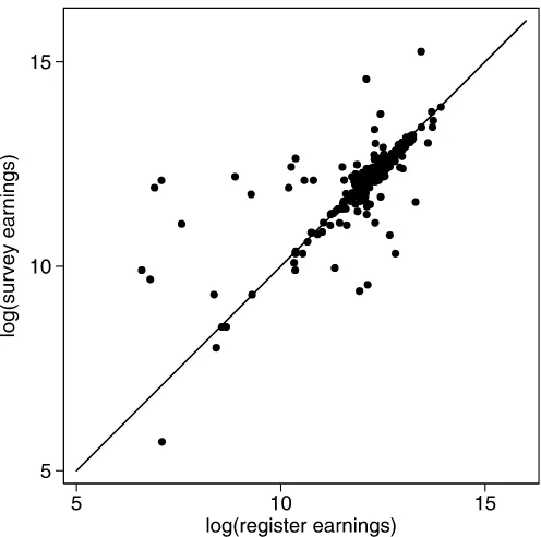
In the Kapteyn–Ypma model, a single latent variable,ξ, rep-resents the true value of the logarithm of earnings of an individ-ual. (We omit the index denoting the individindivid-ual.) This true value is not measured directly; however, two indicators are available, one coming from administrative data and the other coming from individuals’ self-reports collected in a survey. Figure1depicts the observations; the logarithms of the survey earnings are plot-ted against the logarithms of the register earnings. Most points are close to the 45◦line. Thus, for most respondents, earnings as reported in the survey are close to the earnings observed in the administrative records; however, this is not the case for a noticeable number of points.
Figure 1. Survey data versus register data.
Unlike most of the literature in this area, the Kapteyn–Ypma model does not assume that this is necessarily due to measure-ment error in the survey earnings. Rather, Kapteyn and Ypma assume that both indicators may contain error. However, the structure of the error differs between the indicators.
Letξ and three other random variables, ζ,η, andω, be in-dependent of one another and normally distributed with means and variances(μξ, σξ2),(μζ, σζ2),(μη, ση2), and(μω, σω2). Letr denote the value of log earnings from the administrative (regis-ter) data, and letsbe the corresponding value from the survey.
Kapteyn and Ypma (2007) assumed that any errors in the administrative data are due to a mismatch. Letπr be the
prob-ability with which the observed administrative value,r, equals the true value of the respondent’s earnings,ξ. Then 1−πr is
the probability of a mismatch. In case of a mismatch, the ad-ministrative valuercorresponds to the true value of someone else. This mismatched value is denoted byζ. According to the foregoing assumptions,ζ is not correlated withξ. According to the same assumptions, the means and variances ofζ andξ are allowed to differ. This reflects the background of the data collection. The survey data cover only a subset of the popula-tion restricted to individuals age 50 and older and their spouses, but a mismatch may involve an individual from the entire ad-ministrative database, which is a random sample of the entire Swedish population. To formalize this part of the model, the register datarare mixture normal with
r=
ξ with probabilityπr (R1)
ζ with probability 1−πr, (R2)
where the first case reflects a match and the second case reflects a mismatch.
The second part of the model covers the survey data. Three cases are distinguished; earnings are reported without error, with error, or with error and contamination. The probability that the observed survey value is correct is denoted byπs. With
probability 1−πs, the survey data contain response error, part
of which is mean-reverting, as expressed by the termρ(ξ−μξ), where ρ <0 implies a mean-reverting response error in the sense of Bound and Krueger (1991). When the data contain re-sponse error, there is a probability ofπω, that the data are con-taminated, modeled by adding an additional error term,ω. Con-tamination can result from, for example, erroneously reporting monthly earnings as annual or vice versa. Collecting the ele-ments of this second part of the model, the survey datasare mixture normal with
s=
⎧ ⎪ ⎪ ⎪ ⎪ ⎨ ⎪ ⎪ ⎪ ⎪ ⎩
ξ with probabilityπs (S1)
ξ+ρ(ξ−μξ)+η
with probability(1−πs)(1−πω) (S2) ξ+ρ(ξ−μξ)+η+ω
with probability(1−πs)πω. (S3)
Having established the distributions ofr andsseparately, the distribution of(r,s)is a mixture of bivariate normals, with 2×
3=6 classes.
3. THE GENERAL MIXTURE FACTOR ANALYSIS MODEL
As we show in Section6, the Kapteyn–Ypma model is a spe-cial case of a mixture factor analysis model, which has been applied in the literature. Therefore, developing our theory in a generalized form is worthwhile.
Letyn be a vector of observed random variables for
obser-vationn. We assume that there areJtypes or classes of obser-vations, denoted byj=1, . . . ,J. Letπnjbe the (unconditional)
probability that observationnis from classj. In our model,πnj
typically will be strictly between 0 and 1, so that class mem-bership is not known with certainty (although later we discuss known membership as well). In each class, the standard factor analysis (FA) model (e.g., Wansbeek and Meijer2000, chap-ter 7) is assumed to hold under normality. Thus it is assumed that an observation from classjis generated from the model
yn=τnj+Bnjξn+εn, (1)
whereξn∼N(κnj,nj)is a vector of unobserved (latent)
ran-dom variables for observationnandεn∼N(0,nj)is a
vec-tor of random errors that are assumed to be independent ofξn, given the value ofj. The errors may be interpreted as measure-ment errors or disturbances, depending on the application. Our aim is to predictξngiven an observed value ofyn.
The vector of observed variablesyn follows a multivariate
finite mixture distribution, in particular a finite mixture of mul-tivariate normals. Given the FA structure of (1), this is a mixture FA model (e.g., Yung1997). Unlike the standard FA case where observations are routinely centered and thus intercepts play no role, we explicitly incorporate intercepts because they generally will vary across classes and constitute an essential ingredient of the predictors. The parameter vectorsτnjandκnjand matrices
Bnj,nj, andnjare allowed to differ across classes.
We have not attachedjsubscripts toξnandεn, because our
aim is to predictξnand it is conceptually easier if the meaning
of this is the same for all classes. For example, in the Kapteyn– Ypma model,ξncaptures the true value of log earnings, which is defined irrespective of whether earnings are reported with measurement error, whether there is a mismatch of records, or both. However, we allow the distributions ofξnandεnto differ
for different classes, so omitting thejsubscript does not reduce the generality of the model. Applications with class-specific factorsξnj can be incorporated into our notation by stacking
allξnj,j=1, . . . ,J, into the vectorξnand letting the columns
of Bnj corresponding withξnk,k=j, be 0. Our analysis that
follows accommodates rank-deficient matrices, so our setup al-lows for such a specification.
In the notation used so far, we also have allowed the param-eter vectorsτnj andκnj; the parameter matricesBnj,nj, and
nj; and the class probabilities πnj to differ across
observa-tionsn. In a typical application of mixture FA models, the pa-rameters are assumed to be constant within the class, but allow-ing them to be observation-specific includes several models of interest. In particular, this includes all mixtures of linear struc-tural equation models (e.g.,Jedidi, Jagpal, and DeSarbo 1997) and mixtures of linear random coefficient models. These mod-els write the parameters as functions of covariates, of “deeper” parameters, or both; see the supplemental online appendix for further elaboration.
In line with the factor score prediction literature, we assume the parameters to be known and we abstract from estimation is-sues, and thus from issues of identification. Furthermore, we as-sume independence of observations. Consequently, only the ob-served variablesynand observation-specific parameters of
ob-servationnare relevant for our purpose of predicting the latent variableξn. All other observations can be ignored. Therefore, henceforth, we drop the observation indexn. Thus our model for a generic observation from classjis now written as
y=τj+Bjξ+ε, (2a)
ξ∼N(κj,j), (2b)
ε∼N(0,j), (2c)
and the probability that the observation falls in class j is πj.
A direct implication of (2) is
covariance matrixyofy, the meanμξ and covariance matrix ξ ofξ, and the covariance matrixξy of ξ andyfollow by
combining these expressions and the class probabilitiesπj.
4. FACTOR SCORE PREDICTION WITH ONE CLASS
For later reference, we recapitulate some basics of factor score prediction when there is just one class. Given our ear-lier assumptions, all variables are normally distributed in this case, although a large part of the theory of factor score pre-diction still holds under nonnormality (see, e.g., Wansbeek and Meijer2000, section 7.3). We use the same notation as before, but without the class identifierj. Let
ˆ
ξ≡κ+B′−1(y−μ), (4)
F≡−B′−1B. (5)
Using the expression for the conditional normal distribution we obtainξ|y∼N(ξˆ,F). We consider the minimization of the mean squared error (MSE) of a function ofyas a predictor of ξ. Using a standard result in statistics, the MSE is minimized by the conditional expectation. Thus ξˆ is the minimum MSE predictor ofξ.
In general, for reasons of simplicity, we are particularly in-terested in predictors that are linear iny. Because the minimum MSE predictor is already linear in y, imposing the restriction that our minimum MSE predictor is linear leads to ξˆL= ˆξ,
where the subscript L denotes restriction to the class of linear predictors. Later we show that this does not carry over to the mixture model, and that linearity is a binding restriction there.
Now suppose that we view (2) as a linear regression model, with a fixed unknown coefficient vectorξ that we would like to estimate, instead of as a random vector that we would like to predict. Equivalently, consider conditioning on the true value of ξ. [See Anderson and Rubin (1956), for these two views.] Then it follows that the predictorξˆis biased in the sense that
E(ξˆ−ξ|ξ)= −(I−B′−1B)(ξ−κ)=0.
This may be considered a drawback of ξˆ. An unbiased pre-dictor can be obtained as follows. The model, rewritten as y−τ =Bξ+ε, can be interpreted as a regression model with ξ as the vector of regression coefficients,Bas the matrix of re-gressors, andy−τ as the dependent variable. In this model, the generalized least squares estimator is the best linear unbi-ased estimator ofξ, and under normality it is also the best unbi-ased estimator because it attains the Cramér–Rao bound (e.g., Amemiya1985, section 1.3.3). Thus, letting subscript U denote an unbiasedness restriction in the sense of E(ξˆ|ξ)=ξ, and LU, the predictor obtained by imposing both linearity and unbiased-ness, we obtain that
ˆ
ξU= ˆξLU=(B′−1B)−1B′−1(y−τ)
=κ+(B′−1B)−1B′−1(y−μ) (6)
minimizes the conditional MSE, E[(ξˆ−ξ)2|ξ], for every pos-sible value ofξ, conditional on unbiasedness. This implies that it also must minimize the unconditional MSE, E[(ξˆ−ξ)2] =
EE[(ξˆ−ξ)2|ξ], among unbiased predictors, and thus that it is the best unbiased predictor ofξ.
5. A TAXONOMY OF PREDICTORS
With known class membership, the problem of factor score prediction in the mixture FA model reduces to factor score pre-diction in the single class model discussed in the previous sec-tion. The resulting within-class predictors have the same opti-mality properties as in the single class model. In general, class membership is unknown, and there appear to be three natural ways to proceed: (1) compute the within-class predictors for each class and combine them in a weighted average; (2) predict class membership and then use the within-class predictor for the predicted class; and (3) derive predictors that minimize the total mean squared prediction error.
The weighted average is based on the analogy with the means ofyandξ. In these means, the (unconditional) class probabil-itiesπj are the appropriate weights, but for predictors ofξ, we
also can consider usingconditionalclass probabilities giveny. Using Bayes’ rule, these conditional probabilities are
pj(y)≡Pr(class=j|y)=
πjfj(y)
kπkfk(y)
, (7)
wherefj(y)is the normal density with meanμjand variancej,
evaluated iny. We consider both alternatives.
The two-stage predictor would share the desired statistical properties of its second-stage single-class predictor if the pre-diction of class membership in the first stage were error-free. We expect that if class membership can be predicted with a high probability, or if the within-class predictors for the most likely misclassifications in this first stage are very similar, then the two-stage predictor will have desirable properties, such as small MSE.
The system-wide predictors that minimize total MSE apply the methods for deriving single-class predictors to the mixture problem. If we can find solutions to these problems, these are optimal by construction, but their expressions may be compli-cated and finding solutions may not be possible.
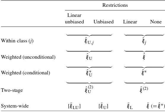
These three general approaches, the unconditional and con-ditional weighting for the weighted predictors and the linear-ity and/or unbiasedness restrictions, lead to an array of predic-tors for the mixture model, which can be grouped into a tax-onomy. The resulting predictors are presented in Table1. The rows indicate the approaches and the type of weighting, and the columns reflect the linearity and unbiasedness restrictions. In Sections5.1–5.4, we systematically develop all of these pre-dictors, although this turns out to be impossible for two of the system-wide predictors (in brackets in the table).
5.1 Within-Class Predictors
The first row of Table 1 presents the predictors from the classes. Because the distribution is normal within a class, the linearity restriction is redundant, as we argued earlier, and just two instead of four predictors are given. We extend the notation of Section4by adding the class subscriptj.
Note that the first predictor,ξˆU,j, is placed under the heading
‘unbiased’ due to reasoning along the lines of a single class; if
Table 1. A taxonomy of predictors in a mixture structural equation model
Restrictions
Linear
unbiased Unbiased Linear None
Within class (j) ξˆU,j ξˆj
Weighted (unconditional) ξˆU ξˆ
Weighted (conditional) ξˆ∗U ξˆ∗
Two-stage ξˆ(U2) ξˆ(2)
System-wide [ ˜ξLU] [ ˜ξU] ξ˜L ξ˜(= ˆξ∗)
classjwere the only class present, then this predictor would be unbiased, but this quality is lost in a multiclass context. It is of interest to elaborate this. From (6),
ˆ
ξU,j=(B′j−j 1Bj)−1B′j−j 1(y−τj)≡B
−
j (y−τj),
where the notationB−j is chosen because it is a generalized in-verse ofBj. Consequently,
E(ξˆU,j|ξ)=B−j
equal toξ for all ξ. This will hold only in special cases. The only case we know of is whenτj andBj do not vary across
classes. The heterogeneity is then restricted to the case where the intercepts and factor loadings are homogeneous, and only the distributions ofξ andεhave a mixture character.
5.2 Weighted Predictors
Given the predictors for a single class, a natural way to pro-ceed to obtain a predictor in the mixture model is to combine the predictors for a single class into a weighted average. Poten-tial weights for these weighted averages are the unconditional class membership probabilitiesπj, by analogy with the mean
ofξ, and the conditional class membership probabilitiespj(y).
The second row of Table1lists the predictors using the uncon-ditional probabilities,
Using the results from Section5.1, we can write
E(ξˆU|ξ)=
j
πjB−j [ ¯τ(ξ)−τj+ ¯B(ξ)ξ]
=B†[ ¯τ(ξ)+ ¯B(ξ)ξ] −τ†,
whereB†=jπjB−j andτ†=jπjB−j τj. Again,ξˆU will be
unbiased only in special cases.
The table’s third row displays the results for weighting with the conditional class membership probabilities. An asterisk dis-tinguishes these predictors from the previous ones. Then
ˆ
Note that the weights depend nonlinearly ony, and thus the lin-earity property is lost when weighting. In addition, the predictor
ˆ
ξ∗Ugenerally will not be unbiased.
5.3 Two-Stage Predictors
An intuitively appealing alternative to computing a weighted predictor is to predict class membership first and then proceed as if class membership were known, using the class-specific predictor of the predicted class. This leads to two-stage predic-tors, analogous to two-step estimators. The obvious class pre-dictor is the class with the highest conditional probability, that is,jˆ≡arg maxjpj(y). Then the two-stage predictors, listed in
the fourth row of Table1, are
ˆ
ξ(U2)= ˆξU,jˆ and ξˆ(2)= ˆξjˆ.
Again, unbiasedness and linearity are lost.
5.4 System-Wide Predictors
The bottom row of Table 1 presents the system-wide pre-dictors obtained by minimizing the MSE with or without the restrictions. Because in the mixture model normality does not hold any longer, linearity is not obtained as a byproduct, and the full range of four different predictors must be considered. We use a tilde to denote system-wide predictors.
Prediction Under Linearity and Unbiasedness. The start-ing point for findstart-ing an unbiased predictor that is linear iny is to find a matrixLand a vector bsuch thatξ˜LU≡L′y+b
should hold for allξ. Because of the (nonlinear) dependence of
¯
τ(ξ)andB(¯ ξ)onξ, a matrixLwith this property exists only in special circumstances. We conjecture that it exists only whenτj
andBjdo not vary across classes. Thus a linear unbiased
pre-dictor generally will not exist. IfτjandBjdo not vary across
classes, then the model can be reinterpreted as a single-class FA model, in which the factors and errors follow nonnormal dis-tributions, particularly mixture normal distributions. Then the minimum MSE linear unbiased predictor follows from the ex-pressions in Section4, which do not depend on normality.
Prediction Under Unbiasedness. Imposing linearity may preclude a solution. We relax this requirement, but maintain unbiasedness. We then consider a predictor ξ˜U=h(y), where h(y)is a function ofysuch that E(h(y)|ξ)=ξ for allξ. Using (8), this requirement forh(y)can be rewritten as
j
πjgj(ξ)E[h(y)|ξ,j] −ξ=0
for all ξ. Attempts to derive the predictor led to expressions without tractable solutions, except for the special case in which τjandBjdo not vary across classes, which was discussed
ear-lier.
Prediction Under Linearity. This case is conceptually the simplest one. It is based on the idea of linear projection. Ac-cording to a well-known result (e.g., Angrist and Pischke2009, theorem 3.1.5 for the univariate case in a slightly different form), the MSE is minimized over all linear functions by
˜
ξL=μξ+ξyy−1(y−μy). (11)
Note that the structure of the model is used only in computing the momentsμξ,μy,ξy, andy. Derivation and optimality
(minimum MSE within the class of linear predictors) of the pre-dictor follow from general principles and do not use the model structure explicitly.
Prediction Without Restrictions. The approach presented here rests on the fact that the MSE is minimized by the mean of the conditional distribution. As with the linear projection re-sult presented earlier, this rere-sult is generic and does not depend on the model’s structure. Of course, for the implementation, we need an expression of this conditional mean, which is derived from the model structure. Adapting results from Section4, we haveξ|y,j∼N(ξˆ
given by (7). Therefore, the system-wide predictor without re-strictions is given by
which equalsξˆ∗, the predictor obtained by weighting of the un-restricted predictors per class using the conditional class prob-abilities. The conditional variance of this predictor is
Var(ξ|y)=
The first term on the right side is the weighted average of the variances within the classes, and the other terms represent the between-class variance.
5.5 Extensions
The derivations up to now assumed that all covariance matri-ces are nonsingular and that extraneous information about class membership is not available. However, in some cases (includ-ing the Kapteyn–Ypma model), these assumptions are not met. In this section we generalize our methods to deal with this sit-uation. In the case of a labeled class, it is known a priori to which class an observation belongs, or this information follows deterministically from the covariates. Thus we have observed (measured) rather than unobserved (unmeasured) heterogene-ity. More generally, we may know that an observation belongs to a certain subset of the classes. This can be viewed as a lim-iting case of observation-specific unconditional class probabil-itiesπnj, and thus is accommodated by our general setup.
Degeneracy denotes singular covariance matrices or factor loading matrices that do not have full column rank. Several types of degeneracies are conceivable in a single-class factor analysis model. For substantive reasons, the errorsε of some of the indicators may be assumed to be identically0, leading to a singular covariance matrix. This also may be the result of
the estimation procedure without a priori restrictions, that is, a Heywood case. Similarly, the covariance matrixof the factors may be singular. Finally, the factor loading matrixBmay not be of full column rank. The latter does not necessarily lead to a de-generate distribution, but it does imply that some of the formu-las presented earlier cannot be applied. In a single-cformu-lass factor analysis setting, singularity of or deficient column rank of Bis not particularly interesting or relevant, because the model is then equivalent to a model with fewer factors and thus can be reduced to a more parsimonious one. However, in a mixture setting, such forms of degeneracy may occur quite naturally. If is nonsingular, then the covariance matrixof the observed indicators is also nonsingular. Thus a necessary condition for singularity ofis singularity of.
The formulas for the single-class predictors cannot be ap-plied directly in the case of degeneracies, because the required inverses may not exist. Furthermore, when there are classes with degenerate distributions of the indicatorsy, (7) does not hold becauseydoes not have a proper density. The supplemen-tal online appendix gives the expressions for the within-class predictors and conditional probabilities in the case of degenera-cies.
With these adapted expressions, prediction of the factor scores is relatively straightforward. For the non–system-wide predictors, we can apply the standard expressions, using the adapted formulas for the within-class predictors and the con-ditional probabilities. For the system-wide linear predictor, (3) is still valid, and thus the predictor ξ˜L is still given by (11),
with−y1replaced by the Moore–Penrose generalized inverse +y if it is singular. The system-wide unrestricted predictorξ˜ is again equivalent to the conditionally weighted unrestricted predictorξˆ∗. We apply these methods in Section6.
6. APPLICATION TO THE KAPTEYN–YPMA MODEL
We can now express the parameters of the general mixture FA model in terms of the parameters of the Kapteyn–Ypma model. We havey=(r,s)′ andκj=μξ andj=σξ2for all classes.
The correspondence between the remaining parameters and the general setup is shown in Table2. A notable feature is thatj
is singular for classes 1–4, so there is a degree of degeneracy in the model (cf. the discussion in Section5.5). Moreover1is
singular, because in class 1,ytakes on values in the subspace y1=y2(i.e.,r=s), whereasjis nonsingular forj=2, . . . ,6.
6.1 Predictors
Given this structure, we now turn to the issue of prediction. We discuss a number of predictors, following the taxonomy pre-sented in Table1.
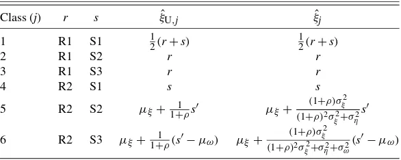
Within-Class Predictors. Formulas for the predictors per class are given in Table3. Note that for classes 5 and 6, the expressions forξˆU,jcan be obtained from the corresponding
ex-pressions forξˆjby settingση2=σω2=0; that is, by ignoring the measurement error variances in the computation.
Weighted Predictors. Moving down the rows of Table1, we obtain overall predictors by weighting theξˆU,j andξˆj with the
probabilitiesπjto obtainξˆU=ar+bs+candξˆ=a′r+b′s+c′,
wherea,b,c,a′,b′, andc′ depend on the various parameters. The detailed expressions can be found in the supplemental on-line appendix.
Table 2. Parameterization of the Swedish earnings data model in terms of a mixture structural equation model
NOTE: R1 indicates correct match; R2, mismatch; S1, no measurement error; S2, measurement error; S3, measurement error and contamination.
Conditionally Weighted Predictors. Consider the eventr=
s. If the observation is drawn from class 1, then the condi-tional probability of observing this event is 1, whereas if the observation is drawn from any of the other five classes, then this conditional probability is 0. Thus the conditional proba-bility thatj=1 given this event is 1:p1((r,r)′)=1 for allr
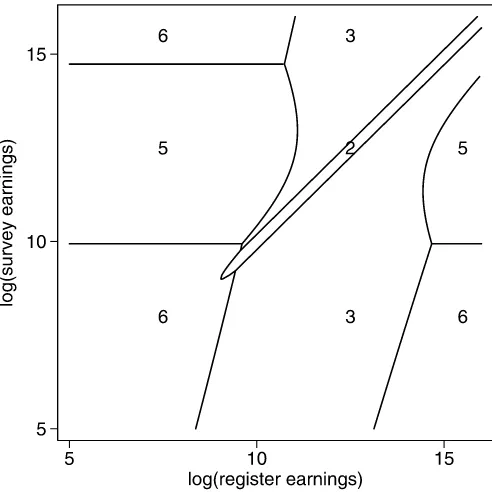
Two-Stage Predictors. In the first stage, class membership is predicted according to the maximum of thepj(y). Thus for
r=s, class 1 is predicted, and for r=s, class 1 is dropped from consideration. Figure2 shows which class is predicted for a given(r,s)combination withr=s. This class predictor was also computed for the observed data points by Kapteyn and Ypma (2007, figure C1). From this figure, we see that close to the 45◦ line, where most of the observations lie in Figure1, membership of class 2 is predicted, and farther away from this
line but still in the middle of the distribution ofr, membership of class 3 is predicted. Perhaps most interesting is the area in the middle-left where membership of class 5 is predicted. There are approximately a dozen points in this area in Figure1, and this is where it is predicted thatris a mismatch. The resulting fac-tor score predicfac-tor is the within-class predicfac-tor corresponding to the predicted class given in Table3.
System-Wide Predictors. The last row of Table1 presents four predictors. As noted in Section5.4, expressions for the two unbiased predictorsξ˜LUandξ˜Ucould not be found. This leaves
us with the projection-based predictor ξ˜L and the conditional
expectation-based predictorξ˜. The expression for the former is given in (11). We need to elaborate the mean and covariance matrices ofyandξ. By weighting the rows of Table2with the π’s, we obtain, after some straightforward algebra, expressions for the elements ofμy,y, andξy. Substitution in (11) again
yields a linear expression, ξ˜L=a′′r+b′′s+c′′. The full
ex-pression for the coefficients is given in the supplemental online appendix. Finally,ξ˜= ˆξ∗, as stated in Section5.4. The formula for the latter has been given by (12).
6.2 Empirical Results
We now turn to the empirical outcomes of the prediction pro-cess using the Kapteyn–Ypma estimates of the model parame-ters. Our objective is to predict earnings by combining the infor-mation from the survey and administrative data. We do so based on a simple model, and on the estimation results obtained from
Table 3. Expressions for the within-class predictors for the Swedish earnings data model as functions of the parameters
Class (j) r s ξˆU,j ξˆj
NOTE: R1 indicates correct match; R2, mismatch; S1, no measurement error; S2, measurement error; S3, measurement error and contamination;s′≡s−μξ−μη.
Figure 2. Predicted class membership jˆ for each combination of register and survey data (excludingr=s).
that model. Kapteyn and Ypma (2007) provided an extensive discussion of their results. Here we only reproduce the relevant parameter estimates that we will use in implementing the var-ious predictors. Estimated means and variances of the normal distributions are given in Table4. The estimates of the other pa-rameters areπr=0.96,πs=0.15,πω=0.16, andρ= −0.01.
Table5presents results per class and the resulting uncondi-tionally weighted predictors. The fourth column gives the class probabilities. The largest class is the second one, represent-ing the case of measurement error, but no mismatch. Columns 5–10 present the numerical results corresponding to Table 3. The predictors in Table3have been written as linear functions, ar+bs+c, ofrands, with the three weightsa,b, andcgiven first forξˆU,jand then forξˆj.
As is apparent from Table3, the rows for classes 5 and 6 are the most interesting ones. These represent cases of mis-match; thus the value from the register is discarded, and only the value from the survey is used, the latter of which suffers from measurement error. If there is no (further) contamination, the unbiased predictor is obtained from the survey figure by slightly overweighting it to compensate for the mean-reverting measurement error. The unrestricted predictor is obtained by slightly downweighting it, because of shrinkage to the overall mean (cf. Wansbeek and Meijer2000, p. 165). If there is con-tamination, then the results diverge strongly. The unrestricted predictor is predominantly a constant, plus some effect from
Table 4. Parameter estimates for the Swedish earnings data model
ξ ζ η ω
μ 12.28 9.20 −0.05 −0.31 σ2 0.51 3.27 0.01 1.52
SOURCE: Kapteyn and Ypma (2007).
the survey, reflecting a large amount of shrinkage due to the large variance of the contamination term, so that more weight is given to the population mean. This phenomenon is sometimes calledborrowing strengthin the random coefficients literature (e.g., Raudenbush et al.2004, p. 9). In contrast, the unbiased predictor is very similar to the predictor obtained when there is no contamination.
The last row of the table gives the results for the predictors
ˆ
ξUandξˆ that are obtained by weighting the preceding rows by
the unconditional class membership probabilities given in the second column. Apart from the constantc, the results from the two predictors differ only from the third digit onward and imply an 89% weight to the register data and an 11% weight to the survey data. The linear projection-based predictorξˆL also can
be expressed as a linear combination ofrands,
˜
ξL=0.22r+0.55s+2.85.
This is a striking result, with very low weight given to the reg-ister data, very unlike the case withξˆUandξˆ.
The predictors discussed so far are all based on uniform weights across the(r,s)space. The conditionally weighted pre-dictors ξˆU∗ and ξ˜ and the two-stage predictors ξˆU(2) and ξˆ(2) cannot be expressed as a simple function ofrands, because the weights now depend on y=(r,s)′ through the densities pj(y), cf. (10). For the two-stage predictors, Figure2indicates
which class-specific predictor is used for a given value of(r,s), and thus the corresponding weights can be found in Table5. Similarly, we can express the conditionally weighted predic-tors as “linear” combinations ofrands, with the weights de-pending on the values ofr and s: ξ˜ = ¯a(y)r+ ¯b(y)s+ ¯c(y), wherea¯(y),b¯(y), andc¯(y)are weighted averages of thea,b, andc coefficients in the last three columns of Table 5, with weightspj(y), and similarly forξˆU∗. We have computed the
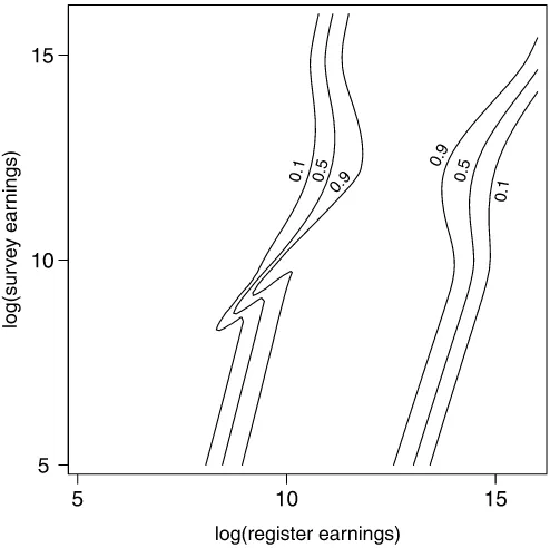
re-sulting relative weight given tor compared withs, computed as a¯(y)/[¯a(y)+ ¯b(y)], over the(r,s)space. The result for ξ˜ is given in Figure3. The figure for ξˆU∗ is very similar and is omitted. We see that in the middle of the figure the predictor is (almost) fully dominated byr, but further from the mean ofξ (μξ =12.28), more weight is attached tos. Because the vari-ance ofζ is large, the relative weight largely depends on the value ofronly and is rather insensitive to the value ofs.
It also is interesting to compare Figure3and Figure2. This comparison shows that in the areas of the(r,s)space where classes 2 or 3 are predicted for the two-stage predictors, which corresponds to these two-stage predictors being equal torand thus giving a 100% weight to r, the relative weight for r in
˜
ξ and ξˆU∗ is also very high, >90%. Conversely, in the areas where class 5 or 6 is predicted for the two-stage predictors,r is predicted to be a mismatch, and its weight in computing the two-stage predictors is 0. In these areas, the relative weight of rinξ˜ andξˆU∗ is very low,<10%. The weight for rinξ˜ and
ˆ
ξU∗changes continuously, whereas it changes discretely for the two-stage predictors, but Figure3shows that “continuously” is still quite fast, so that the two-stage predictors and conditionally weighted predictors are very similar.
To obtain an overall comparison of the performance of the seven predictors, we computed their reliabilities. The reliabil-ity of a proxy is a measure of the precision with which it mea-sures the latent variable of interest. Whenξ is one-dimensional,
Table 5. Unconditional class membership probabilities for the Swedish earnings data model and predictors as linear expressionsar+bs+c
ˆ
ξU,j ξˆj
Class (j) r s πj a b c a b c
1 R1 S1 0.15 0.5 0.5 0 0.5 0.5 0
2 R1 S2 0.69 1 0 0 1 0 0
3 R1 S3 0.13 1 0 0 1 0 0
4 R2 S1 0.01 0 1 0 0 1 0
5 R2 S2 0.03 0 1.01 −0.11 0 0.99 0.12
6 R2 S3 0.01 0 1.01 0.19 0 0.25 9.32
ˆ
ξU: 0.89 0.11 −0.00 ξˆ: 0.89 0.11 0.05
NOTE: R1 indicates correct match; R2, mismatch; S1, no measurement error; S2, measurement error; S3, mea-surement error and contamination. Probabilities do not sum to 1 because of rounding.
the reliability of a proxyxis the squared correlation betweenξ andx. The reliability of a linear combinationx=ar+bs+c can be obtained straightforwardly in closed form. For the condi-tionally weighted and two-stage predictors, reliabilities cannot be computed analytically because they are nonlinear combina-tions ofrands. We computed the reliabilities of these predic-tors by simulating 100,000 draws from the model and comput-ing the squared sample correlation between factor and predic-tor from these. (We also computed the reliabilities of the lin-ear proxies using these draws, which corresponded closely to the results obtained from the closed-form expressions for these proxies.)
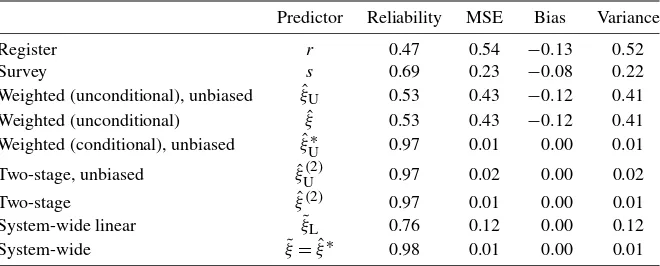
The results are given in Table6for the seven predictors con-sidered throughout, plusrandsas a reference. The table also reports the (unconditional) MSEs of the predictors, MSE=
E(predictor−ξ )2, which are of course strongly negatively re-lated to the reliabilities, although they are not perfect
substi-Figure 3. Relative weight of log(register earnings)rin the condi-tionally weighted predictorξ˜. The lines connect points with the same relative weight given tor, computed asa¯(y)/[¯a(y)+ ¯b(y)].
tutes. For example, unlike the reliability, the MSE of a linear combinationx=ar+bs+cdepends on the constantc. In addi-tion, the table presents the (unconditional) bias E(predictor−ξ ) and (unconditional) variance Var(predictor−ξ )of the predic-tion errors.
The table presents some striking results. The register datar have a squared correlation with the true log earningsξ of<0.5. Informally stated, r is a clear loser, which is surprising. Ap-parently a high probability of being exactly correct is not suf-ficient, and the small probability of being an independent draw from a different distribution has dramatic consequences for the statistical properties of the indicator. The survey datasperform considerably better thanr. The predictors obtained by uncon-ditional weighting per class perform poorly, and the predictor based on linear projection performs much better. However, all predictors that use the conditional class membership probabili-ties are nearly perfect (withξ˜performing marginally better than the others), again, of course, against the background of the pos-tulated model.
As shown in the last two columns of Table6, the biases of the first four predictors are sizeable, but the squared biases are negligible compared with the variances, so that the variances dominate the MSEs. It is also noteworthy that bothrandshave negative bias. The bias ofris due to mismatch, whereas the bias ofsis due to the negative means of the measurement errorηand contaminationω. The biases ofrandsare identified based on ther=scases, which are higher up on the earnings distribution (on average) than the other cases.
The excellent performance in terms of reliability and MSE of the two-stage predictor, both in an absolute sense and com-pared with the minimum MSE predictorξ˜, is related to the high probability with which class membership is correctly predicted. Overall, the probability of correctly classifying an observation is 96%. Among the misclassifications, a classification of an ob-servation from class 3 as an obob-servation from class 2 takes more than 2 percentage points of the remaining 4 percent. But be-cause the within-class predictor isrin both class 2 and class 3, this has no consequence for the precision of the two-stage pre-dictors. We expect that in situations where the class probabil-ities are less concentrated and the within-class predictors vary more widely across classes, the two-stage predictors will be no-tably less precise.
Table 6. Precision of the predictors
Predictor Reliability MSE Bias Variance
Register r 0.47 0.54 −0.13 0.52
Survey s 0.69 0.23 −0.08 0.22
Weighted (unconditional), unbiased ξˆU 0.53 0.43 −0.12 0.41 Weighted (unconditional) ξˆ 0.53 0.43 −0.12 0.41 Weighted (conditional), unbiased ξˆU∗ 0.97 0.01 0.00 0.01
Two-stage, unbiased ξˆU(2) 0.97 0.02 0.00 0.02
Two-stage ξˆ(2) 0.97 0.01 0.00 0.01
System-wide linear ξ˜L 0.76 0.12 0.00 0.12
System-wide ξ˜= ˆξ∗ 0.98 0.01 0.00 0.01
7. DISCUSSION
In this article we have addressed a very simple question: When we are given two numerical values for the same quantity, which often are not equal, what is the best guess as to the truth? As always, getting to a sensible answer involves some model building, necessarily based on some assumptions. The model in this case was of the mixture factor analysis type, and answering our question amounted to factor score prediction in that model. Because that topic was apparently hardly researched, we first derived the methods needed. Taking the standard factor score prediction literature as our point of departure, we systematically explored the options for constructing predictors for the mixture case. This produced seven predictors for further consideration.
We then explored the consequences of two extensions of the model. The first extension is the presence of labeled classes, which means that class membership is either known a priori or is a deterministic function of the covariates. The second exten-sion is the incorporation of degenerate distributions and rank-deficient coefficient matrices in the model.
We applied the tools that we developed to the case of Swedish earnings data, where measurements were available for each in-dividual both from an administrative database and from a sur-vey. We took the Kapteyn–Ypma model (Kapteyn and Ypma 2007) as given, including their parameter estimates, and stud-ied prediction of true (log) earnings from the two observed mea-surements. The major conclusion is that conditionally weighted predictors and the two-stage predictors perform extremely well, much better than either the register data or the survey data by themselves, predictors based on unconditional weights, or the linear-projection-based predictor.
A topic for further research is the generality of our empirical findings. In particular, researchers increasingly use administra-tive data matched to surveys and simply treat the administraadministra-tive data as if they contained the correct values. Our empirical re-sults show that if there is a potential for mismatch, then this approach might be counterproductive, because we showed that in the Kapteyn–Ypma model, the survey earnings have a higher reliability and lower MSE than the register earnings.
In the U.S., administrative data from the Social Security Ad-ministration (SSA) provide a primary source of such matched data sources. These data have been matched to nationally rep-resentative surveys, such as the Health and Retirement Study (HRS), Survey of Income and Program Participation (SIPP), and the Current Population Survey (CPS). The algorithm that
the SSA uses for matching administrative records to survey records tends to be conservative in declaring a correct match, but it certainly is not guaranteed to be error-free. Given the findings presented in this article, it seems worthwhile to study the prevalence of mismatches using a model like the Kapteyn– Ypma model and their potential consequences using an analysis like the one in this article.
There remains the question of why the register data perform so poorly. It is beyond the scope of this article to resolve this puzzle. A speculative explanation may be that in the Kapteyn– Ypma model, the register data are assumed to deviate from the true earnings values only in case of a mismatch, but these data might contain some measurement error, possibly in the case of unreported earnings from a second or third job. Failure to report these earnings could be related to the earnings being minor or pertaining to unreported employment in the underground econ-omy (see Kapteyn and Ypma2007, footnote 5, for a similar ex-ample). If this were the explanation, then “mismatch” should be reinterpreted as “misreport.” Under such a reinterpretation, the model specification likely would need to be changed slightly, because then register earnings under misreporting would not be independent of the true earnings. However, it is not immediately clear whether they would be positively or negatively correlated with true earnings, and thus whether the reliability of register earnings as a measure of true earnings would be higher or even lower than estimated in this article. In any case, it seems that even under the most favorable circumstances, the quality of the register data is lower than is typically assumed in validation studies.
SUPPLEMENTARY MATERIALS
Measurement error in earnings data: using a mixture model approach to combine survey and register data: Supple-mental online appendix: Contains additional material, as referenced in the main text. This shows the generality of the model; shows that several models discussed in the lit-erature are special cases of our model; gives detailed for-mulas for single-class prediction with degenerate distribu-tions; gives a detailed treatment of conditional probabilities in mixture models with degenerate distributions; and gives detailed formulas for the predictors in the Kapteyn–Ypma model. (supplement.pdf)
ACKNOWLEDGMENTS
The authors thank Jelmer Ypma and Arie Kapteyn for shar-ing their code and for discussions about their model, and Jos ten Berge and conference participants at Aston Business School, Birmingham (in particular Battista Severgnini) for stimulating discussions and comments on an earlier version of this article. They also thank the editors (Arthur Lewbel and Keisuke Hi-rano), an associate editor, and a referee for helpful comments. The National Institute on Aging supported the collection of the survey data and subsequent match to administrative records (grant R03 AG21780). Rohwedder acknowledges financial sup-port from NIA grant P01 AG08291.
[Received June 2008. Revised February 2011.]
REFERENCES
Amemiya, T. (1985),Advanced Econometrics, Cambridge, MA: Harvard Uni-versity Press. [194]
Anderson, T. W., and Rubin, H. (1956), “Statistical Inference in Factor Anal-ysis,” inProceedings of the Third Berkeley Symposium on Mathematical Statistics and Probability V, ed. J. Neyman, Berkeley: University of Califor-nia Press, pp. 111–150. Available athttp:// projecteuclid.org/ euclid.bsmsp/ 1200511860. [193]
Angrist, J. D., and Pischke, J.-S. (2009),Mostly Harmless Econometrics: An Empiricist’s Companion, Princeton, NJ: Princeton University Press. [196] Bound, J., and Krueger, A. B. (1991), “The Extent of Measurement Error in
Longitudinal Earnings Data: Do Two Wrongs Make a Right?”Journal of Labor Economics, 9, 1–24. [191,192]
Bound, J., Brown, C., and Mathiowetz, N. (2001), “Measurement Error in Sur-vey Data,” inHandbook of Econometrics, Vol. 5, eds. J. J. Heckman and E. Leamer, Amsterdam: North-Holland, pp. 3705–3843. [191]
Jedidi, K., Jagpal, H. S., and DeSarbo, W. S. (1997), “Finite-Mixture Struc-tural Equation Models for Response-Based Segmentation and Unobserved Heterogeneity,”Marketing Science, 16, 39–59. [193]
Kapteyn, A., and Ypma, J. Y. (2007), “Measurement Error and Misclassifica-tion: A Comparison of Survey and Administrative Data,”Journal of Labor Economics, 25, 513–551. [191,192,197,198,200]
Pischke, J.-S. (1995), “Measurement Error and Earnings Dynamics: Some Es-timates From the PSID Validation Study,”Journal of Business & Economic Statistics, 13, 305–314. [191]
Raudenbush, S. W., Bryk, A. S., Cheong, Y. F., and Congdon, R. (2004),
HLM 6: Hierarchical Linear and Nonlinear Modeling, Chicago: Scientific Software International. [198]
Wansbeek, T. J., and Meijer, E. (2000),Measurement Error and Latent Vari-ables in Econometrics, Amsterdam: North-Holland. [193,198]
Yung, Y.-F. (1997), “Finite Mixtures in Confirmatory Factor-Analysis Models,”
Psychometrika, 62, 297–330. [193]
Zhu, H.-T., and Lee, S.-Y. (2001), “A Bayesian Analysis of Finite Mixtures in the LISREL Model,”Psychometrika, 66, 133–152. [191]