Full Terms & Conditions of access and use can be found at
http://www.tandfonline.com/action/journalInformation?journalCode=ubes20
Download by: [Universitas Maritim Raja Ali Haji] Date: 12 January 2016, At: 00:27
Journal of Business & Economic Statistics
ISSN: 0735-0015 (Print) 1537-2707 (Online) Journal homepage: http://www.tandfonline.com/loi/ubes20
Deducing the Implications of Jump Models for the
Structure of Stock Market Crashes, Rallies, Jump
Arrival Rates, and Extremes
Gurdip Bakshi, Dilip Madan & George Panayotov
To cite this article: Gurdip Bakshi, Dilip Madan & George Panayotov (2010) Deducing the Implications of Jump Models for the Structure of Stock Market Crashes, Rallies, Jump Arrival Rates, and Extremes, Journal of Business & Economic Statistics, 28:3, 380-396, DOI: 10.1198/ jbes.2009.06176
To link to this article: http://dx.doi.org/10.1198/jbes.2009.06176
Published online: 01 Jan 2012.
Submit your article to this journal
Article views: 98
Deducing the Implications of Jump Models for
the Structure of Stock Market Crashes, Rallies,
Jump Arrival Rates, and Extremes
Gurdip B
AKSHISmith School of Business, University of Maryland, College Park, MD 20742 ([email protected])
Dilip M
ADANSmith School of Business, University of Maryland, College Park, MD 20742 ([email protected])
George P
ANAYOTOVMcDonough School of Business, Georgetown University, Washington, DC 20057 ([email protected])
This article studies the structure of stock market crashes, rallies, their jump arrival rates, and extremes. Large market moves are characterized in a pure-jump modeling framework. Based on both raw and de-volatized returns, it is shown empirically that crashes are more severe in intensity than rallies, and have higher arrival rates. At the same time, both left-tail and right-tail extreme events conform with Fréchet limit laws. Pure-jump models which describe well the tail properties of market returns are identified via their Lévy measures. The distribution of extreme events implied by our model’s Lévy measure is closer to the actual realization of extremes than those of competing models. Finally, there is information content in the Lévy measure of pure-jump models for forward arrival rate of jumps.
KEY WORDS: Arrival rates; Crashes; Extremes; Jump structure; Lévy measure; Limit laws; Pure-jump price processes; Rallies.
1. INTRODUCTION
The purpose of this article is to examine the structure of stock market crashes, rallies, their arrival rates, and extremes. We characterize large moves in a pure-jump modeling framework, and we show empirically that pure-jump models can more aptly capture the tail properties of market returns. Compared to the extant literature, we make contributions in several dimensions by addressing four questions: Have equity markets experienced a higher number of crashes than rallies? How distinct are the left- and right-tails of market returns? Are they governed by different limit laws? What properties must be shared by a the-oretical model class to match the patterns of observed market extremes and the arrival rate of jumps?
At the center of financial economics is the model of Merton (1976), who treated stock prices as jump-diffusions with Pois-son intensity of jumps and Gaussian jump distribution. Jump-diffusions possess the feature that their path is continuous ex-cept for occasional discontinuities. While jump-diffusions have proved flexible in modeling large perturbations, they are sus-ceptible to the drawback that the densities of the diffusion com-ponent, that surrogates small moves, and of the jump compo-nent, that surrogates large moves, are analytically detached. As a possible remedy, we exploit a parsimonious one-dimensional Lévy pure-jump model for market returns. Such pure-jump models are suited for our study since they can generate asym-metric jump arrival rates and jump sizes, which allow for a bet-ter differentiation between the left- and the right-tail. Economic and statistical considerations that argue for pure-jump stock price models can be found in Madan and Seneta (1990), Eber-lein and Keller (1995), Barndorff-Nielsen (1998), Madan, Carr, and Chang (1998), Barndorff-Nielsen and Shephard (2001),
Eberlein (2001), Carr et al. (2002), Huang and Wu (2004), Cont and Tankov (2004), Wu (2006), Bakshi, Carr, and Wu (2008), Aït-Sahalia and Jacod (2008), Li, Wells, and Yu (2008), Jacod and Todorov (2009), and Todorov (2009).
In contrast to classic models, the source of randomness in our model is a Brownian motion evaluated at a gamma direct-ing process (e.g., see, among others, Madan and Seneta1990; Conley et al.1997; Madan, Carr, and Chang1998; and Carr and Wu2004). The directing process can be motivated by informa-tion arrival, represented by some measure of economic activity. For instance, it is volume in Clark (1973), number of trades in Ané and Geman (2000), and volatility in Carr et al. (2003) and Barndorff-Nielsen and Shephard (2006). Intuitively, a Brown-ian motion law in economic time instead of calender time pro-vides the economic underpinnings for the model. The resulting price process (i) has non-Gaussian local increments, (ii) is pure-jump, devoid of any continuous martingale components, and (iii) possesses a tractable return characteristic function with fi-nite moments of all orders. More distinctively, by appealing to the Lévy–Khintchine theorem, the Lévy measure is derivable in analytical closed-form. Special to our theoretical framework, the Lévy measure controls the arrival rate of jumps over the entire continuum; whether large or small and whether negative or positive. Conforming with the observed dynamics of crashes and rallies, the higher the jump size, the lower are the respective jump arrival rates. Based on the parametric form of the Lévy
© 2010American Statistical Association Journal of Business & Economic Statistics July 2010, Vol. 28, No. 3 DOI:10.1198/jbes.2009.06176
380
measure, the distribution of the largest percentage price fluctu-ation is derived analytically. Furthermore, it is shown that the returns process in our theoretical model is in the domain of at-traction of the fat-tailed Fréchet limit law.
Our empirical investigation employs daily data on the Dow Jones Industrial Average (DJIA) from the beginning of 1897 to the end of 2007, and we use both raw and devolatized returns. Return devolatization can be motivated by the many studies that show strongly time-varying volatility (e.g., Nelson1991; Bollerslev, Chou, and Kroner1992; and Engle2004), and al-lows us to reconcile our focus on Lévy return models, implying independent and time-homogeneous increments, with the ob-served properties of stock returns data. To see that devolatiza-tion can highlight tail events, consider the significance of the −3.35% drop in the DJIA on March 27, 2007, in terms of de-volatization. Given that the post 1946 daily volatility is around 0.9%, this single-day drop materializes into a 3.8-sigma event in the raw returns data. At the same time, devolatization accen-tuates the raw move into a−7.56% drop, which translates into a 8.4-sigma event. In fact, it is one of the five largest drops in the devolatized time series post 1946.
Based on raw returns, we find that the probability of a daily stock market decline in excess of 5% is nonnegligible; about 0.25%. There are 69 days on which the stock market has dropped by more than 5%. But a market rally of 5% or higher is observed only 52 times. Moreover, market crashes are not only more likely to occur than rallies with higher crash arrival rates, but are substantially more severe. The pre 1946 crash valuation measures depart radically from the post 1946 counterpart with the left-tail decaying to zero much slower than the right-tail. To emphasize further the distinction between the two tails, we construct a time series of left- and right-tail events measured by the maximum daily absolute percentage decline and the maxi-mum daily percentage rise, respectively, over fixed block sizes. We find a positive spread between the left-tail and right-tail ex-tremes when the block size is 42, 84, and 126 days. Many of the features of raw returns are more pronounced in devolatized returns.
Next we examine whether the structure of jumps implied by our model is consistent with the arrival rates of jumps of various sizes, as observed in the data. When the log arrival rate of jumps is regressed on a constant, the jump size, and the log jump size, as specified by the functional form of the log Lévy measure in our model, there are no violations of the restriction that each estimated coefficient be negative. In contrast, the Cox and Ross (1976) jump-model with log Lévy measure that is quadratic in the jump size, and the Das and Foresi (1996) and Kou (2002) models with log Lévy measure that is linear in the jump size are both rejected in our performance horse-races. Further test of empirical specification uncovers the finding that our model is consistent with the Carr et al. (2002) model.
Relying on the Fisher–Tippett theorem we investigate the limit laws of extremes. Estimation results show that both left-tail and right-left-tail extremes have limiting Fréchet distributions. Consistent with the observed pattern of the extremes, the es-timated parameters of the Fréchet densities imply that crashes are more probable than rallies, and post 1946 markets are less inclined to extreme fluctuations. The Fréchet tail-indexes reveal that the distribution of right-tail events has thinner tails than that
of the left-tail events. Supporting the viability of our pure-jump modeling framework from another perspective, we also find that returns simulated from the model exhibit limit law properties that bear resemblance to actual return data.
Finally, motivated by the notion that Lévy measures are suffi-cient (in theory) to pin down the arrival rate of jumps, we pursue an empirical specification to assess whether there is information content in the Lévy measure, estimated in an earlier period for jump arrival rates in a later period. Predictive regressions reveal that the current Lévy measure contains information for forward arrival rates.
This article is organized as follows. Section 2 develops a pure-jump representation of the price process. We present the Lévy measure of the model and all other models used in the em-pirical investigation. Section3describes the procedure applied to devolatize returns. Section4 highlights features of crashes and extremes in the stock market and the structure of jump ar-rival rates. The purpose of Section5is to validate models based on their consistency with the observed jump arrival rates and jump sizes. Section6reports our findings on the limit laws of extremes constructed from left-tail and right-tail events based on devolatized returns as well as those from simulated returns. Plausibility of the tail probability model is evaluated through a predictive exercise in Section7. Conclusions are in Section8.
2. MODEL OF MARKET CRASHES, RALLIES, JUMP ARRIVAL RATES, AND EXTREMES
Fix the probability space as (,F,P). Unless stated other-wise, all conditional expectations,Et(·), are taken under the ob-jective probability measure and according to the filtration gen-erated byFt. Denote the per share price of the market index by
{S(t),t∈ [0, ϒ]}and the logarithmic rate of return as
R(0,t)≡lnS(t)−lnS(0). (1) To preserve tractability of theoretical analysis, we maintain the assumption of stationary and independently distributed returns and, hence, adopt a Levy process to model index returns. How-ever, in the empirical investigation of model implications we adjust our data for variations in return volatility.
Our treatment of market crashes and rallies essentially in-corporates jumps in market index returns. Assuming that the continuous-time price process has a left limit and is right con-tinuous, we formally define a jump of any size in the market index as in Merton (1976):
z(u)≡lnS(u)−lnS(u−), z(u)∈(−∞,+∞). (2) We note that in our modeling setup jumps occur at inaccessible (surprise) times and the probability of a jump at any fixed time is zero.
Furthermore, the biggest positive or negative jump that oc-curs over any fixed interval(0,b)is a well-defined object. De-fine the entities
which, respectively, represent the absolute value of the largest instantaneous percentage price decline and the largest percent-age rise in the stock price.Mb−captures the worst possible in-stantaneous loss for a long investor andMb+captures the worst possible instantaneous loss for a short investor.
The entities defined in Equations (3) and (4) allow us to for-malize a framework for modeling the extreme return fluctua-tion, whether positive or negative. Our theoretical interest lies in studying the laws Prob(Mb−≥K)and Prob(Mb+≥K)for
K>0. Abstracting from the specific parent distribution gov-erning local fluctuations in returns, limit laws of the extremes will be obtained in the sense of Fisher and Tippett (1928) (see also Kendall and Stuart1977and Embrechts, Kluppelberg, and Mikosch1997).
2.1 Pure-Jump Return Dynamics
We focus on one-dimensional Lévy (pure-jump) processes in modeling market returns. The hallmark of a pure-jump model is that its path is nowhere continuous and every move consti-tutes a jump. Our contention is that pure-jump models gener-ate asymmetric jump arrival rgener-ates and jump sizes, which allow for a better differentiation between the left- and the right-tail. That is, they offer the versatility to capture diverse tail prop-erties of market returns. Furthermore, they present a parsimo-nious alternative to jump-diffusions in modeling extreme mar-ket moves. Note that the proposed pure-jump model shares an important property with diffusions, which, at the same time is not exhibited by jump-diffusions. Diffusions are associated with Gaussian limit laws. In a similar way, pure-jump models of the class considered are associated with infinitely divisible limit laws, hence, they generalize over the Gaussian local law of motion, but preserve the limit law property. In contrast, it is provable that jump-diffusions do not satisfy the limit law. Specifically, the generic property of limit law that|z|(z), for Lévy measure(z), be decreasing forz>0 and|z|(z)be in-creasing forz<0, does not hold for the jump diffusion model of Merton (1976).
Following Madan and Seneta (1990), Madan, Carr, and Chang (1998), and Carr et al. (2002), let the market index
a standard Brownian motion evaluated at a random (gamma) timey(t). Realize thatB(t1)andB(t2)are correlated, but that does not imply return predictability, as return is modeled as the difference and, hence, is not autocorrelated. While the level of
B(t2) is predictable, givenB(t1), the increment B(t2)−B(t1)
is unpredictable. Here y(t)governs the evolution of the time-change or the directing process. Refining the diffusion para-digm, the second source of randomness is obtained by superim-posing stochastic time-changes on a standard Brownian motion. Intuitively, the random timey(t)can be abstractly thought as representing aggregate economic activity and is, thus, distinct from calender time. However, the attributes of subordination in our model are different from others: it is lognormally dis-tributed volume in Clark (1973), it is number of trades in Ané and Geman (2000), and it is volatility in Carr et al. (2003) and Barndorff-Nielsen and Shephard (2006). Absent economic ac-tivity, there is no time change. Thus, we have the Brownian motion law in economic time rather than in calender time.
In our approach,g(t)is a stand-in for the variance-gamma process (e.g., Madan, Carr, and Chang1998). LetB(t)andy(t)
be independent for all t. Conditional on y(t), the stochastic process g(t) is distributed normal with meanθy(t) and vari-anceσ2y(t). This model structure facilitates simulation of the increments of the process over intervalt:g(t+t)−g(t)= (θy)t+σ√yz˜√t, where˜zisN(0,1)andy∼Gamma (see Ribeiro and Webber2003). The characteristic function ofg(t)
is moments of the return distribution and the sign of skewness in the market return is the same as that ofθ. The compensator
ω=1κln(1−θ κ−
1 2κσ
2)in Equation (5) is there to guarantee that the drift of the market indexμsatisfiesE0(S(t))=S0eμt.
The continuous-time price process in Equation (5) is con-ceptually and theoretically attractive. First, the price process posited in Equation (5) is a semimartingale and consequently arbitrage-free. It inherits from traditional models the trait that the return distribution has well-defined algebraic moments up to all orders. Additionally, as the time change is distributed gamma, the return distribution is stable under additivity.
By relying on the return specification Equation (5) and the characteristic function in Equation (8), the return characteristic functionFR(0,t;φ)≡E0(eiφR(0,t))takes the form
which is crucial for deriving the structure of jumps by ap-plying the Lévy–Khintchine integral representation of the log characteristic function. It follows from Equation (9) that
FR(0,t;φ)=exp(−t(φ)), where (φ) is the characteristic exponent, hence, the returns process also has independent and time-homogeneous increments.
R(0,t)is normal, it follows that the transition density function,
(R(0,t)), is
whereKa(b)represents the modified Bessel function of the sec-ond kind,υ≡κt−12, andβ≡θ2+2σκ2. Based on Equation (10) it may be verified from Johnson, Kotz, and Balakrishnan (1994) that the stock price relative,
exp(R(0,t))−1≡r(0,t)∼Loggamma. (11) In principle, one can rely on the density function in Equa-tion (10) or the transformed density forr(0,t)for implementing the pure-jump model.
The price process in Equation (5) is (i) locally non-Gaussian and (ii) a pure-jump process with no continuous martingale components. This can be verified by observing that any continu-ous price process with a finite variance rate is locally Gaussian (e.g., Revuz and Yor1991), which the price process in Equa-tion (5) fails to satisfy. The absence of a continuous martingale component is not critical as small jumps of highly active jump processes can closely mimic diffusion dynamics (Aït-Sahalia and Jacod2009). In fact, such small jumps are often simulated by a Gaussian component.
2.2 The Lévy Measure and the Structure of Jumps
Associated with each continuous-time stochastic jump pro-cess of homogeneous independent increments is a Lévy mea-sure that governs the instantaneous arrival rate of jumps of all sizes, whether negative or positive. As previously defined, letz
denote the size of the instantaneous jump in the log price. Since
z>0 orz<0, denote the Lévy measure of positive jumps by
+(z)and the negative counterpart by−(z).
2.2.1 Parametric Form of the Lévy Measure. Applying the Lévy–Khintchine Theorem (Jacod and Shiryaev 1987; Bertoin1996; and Sato1999) to the present pure-jump model, the Lévy measures+(z)and−(z)satisfy
Substituting the return characteristic function in Equation (9) into Equation (12) and setting̺=μ+κ1ln(1−θ κ−12κσ2), we obtain the Lévy measure (hereby, LM)
(z)=
The LM postulated in Equation (13) is central to our frame-work. Since 0+∞+(z)dz=0
−∞−(z)dz= +∞, the LM is consistent with infinitely many jumps per unit time. But
if jumps of size less than ǫ (say, the minimum tick size) are excluded, both ǫ+∞+(z)dz and −∞−ǫ −(z)dz stay fi-nite. One may then interpret +(z) as the instantaneous ar-rival rate of positive jumps of size zwith conditional density
+(z)/ǫ+∞+(z)dz and a jump having occurrence proba-bilityǫ+∞+(z)dz(properly normalized). Clearly, the arrival rate of positive (negative) jumps of size greater than K must be: K+∞+(z)dz [−∞−K−(z)dz]. Furthermore, as the sto-chastic process of the arrival of jumps of size z>K is Pois-son, the probability of no (instantaneous) arrival of the jump is exp(−K+∞(z)dz).
In short, the LM embodies complete probabilistic informa-tion about the arrival rate of jumps, both positive and negative. There is a relationship between the arrival rates of small and large moves, but not in the occurrence of events as the moves are occurring at inaccessible times. Thus, there is no causal re-lation between small and large events.
The LM in Equation (13) is downward-sloping with ∂(∂zz)=
all zand for all j, and implies the coexistence of high arrival rates of small jumps (positive or negative) and the low arrival rates of large jumps.
Whenθ=0, the LM assigns an unequal weight to the arrival of negative versus positive moves, i.e., ǫ+∞+(z)dz can be higher or lower than∞−ǫ−(z)dz. Thus, it is possible to rec-oncile that (i) positive jumps overall have higher arrival rates than negative jumps, and (ii) big positive jumps possess lower arrival rates compared to big negative jumps (the crash proba-bility is higher).
Before proceeding, recall from theorem 5 in Clark (1973) that the return characteristic function is not in analytical closed-form. Consequently, the Lévy–Khintchine integral representa-tion is not solvable, and hence the Lévy measure and the struc-ture of price jumps cannot be recovered. For this reason, Clark’s model of time-changes is of limited value in studying jump ar-rival rates and extremes.
2.2.2 Lévy Measures for Competing Models. To put the main ideas in perspective, consider first the classic Merton (1976) jump-diffusion model where uncertainty is driven by a diffusion component and an orthogonal jump component:
dS(t) with intensity λJ. Setting diffusion volatilityσ =0 results in the Cox and Ross (1976) jump model: dSS((tt))=J(t)dq(t). Given that its return characteristic function is exp(λJt[exp(iφln(1+
μJ)−12iφσJ2+12(iφ)2σJ2)−1]), we apply the Lévy–Khintchine representation in Equation (12) and deduce the Lévy measure
CR(z)=λJ
which is the probability of a Poisson jump multiplied by the density of the percentage jump size. It also represents the Lévy measure of the Merton (1976) model.
Departing from Merton (1976) and Cox and Ross (1976), the model of Das and Foresi (1996) considered an exponential dis-tribution alternative forJ(t). With Bernoulli probability of pos-itive (negative) jumps being ϑ (1−ϑ), the analytical form of the Lévy measure is
DF(z)=
+(z)≡ϑ ςe−ςz ifz>0
−(z)≡(1−ϑ )ςe−ς|z| ifz<0, (17) for some constantςof the exponential distribution. The model of Kou (2002) shares the same lineage as Equation (17), and the Lévy measure of both models is nested within Equation (13).
Of possible interest in our context are models where the ar-rival rate of jumps are not only linked to jump density, but are also regulated by a random diffusion component. To be precise, suppose one takes the model of Merton (1976) and Cox and Ross (1976) and adopts a modification where the Poisson intensity of jumps is a stochastic process (maintain-ing Gaussian jump distribution). In the option model of Bates (2000), for instance,dq(t)=1, with Probability(dq(t)=1)=
λ(t)dt=(λ0+λvV(t))dt, whereV(t)follows a square-root dif-fusion process with linear drift. Hence,λ(t), which is a con-stant in Merton (1976) and Cox and Ross (1976), is linear in diffusive volatility. The arrival rate of jumps takes the form:
(λ0+λvV(t))exp(−(z−ln(1+μJ)+12σJ2)2/(2σJ2)). A like-wise attribute is shared by the model of Santa-Clara and Yan (2009), whereλ(t)is quadratic in latent volatility. See Carr et al. (2003) for another model class where the arrival rate of jumps of sizezis represented by(λ0+λvV(t))( z), and( z) repre-sents Lévy jump density. The overall impact of such models is to enhance jump activity for both small and large jump sizes in volatile markets. These models, thus, introduce another layer of complexity where the volatility process must be parameterized, and are outside of our present empirical scope.
Finally, Carr et al. (2002) have generalized the Lévy measure in Equation (13) to
If ξ <0, it supports finite activity. On the other hand ξ >0 implies infinite activity, andξ >1 implies infinite variation. If
ξ=0, we recover the Lévy measure of Equation (13).
Although appealing in their own right, we choose not to pur-sue three other pure-jump models in the interest of brevity. The first model is the generalized hyperbolic model (Eber-lein, Keller, and Prause 1998). Its Lévy density is expressed in modified Bessel functions of the first and second kind. Sec-ond, from equation (2.9) in Barndorff-Nielsen (1998), the Lévy measure of the Normal Inverse Gaussian model is:NIG(x)=
δζexp(βz)K1(ζ|z|)
π|z| , for some parameters ζ, δ >0, and β and Kν(·)is the modified Bessel function of the second kind. The
third model is the infinite variation model of Schoutens (2003), which has Lévy measure:Meixner(z)=δzexpsinh(β(πz/ζ )z/ζ ), for para-metersζ >0,|β|< π, andδ >0.
Lévy measures for the candidate models derived in Equations (13), (16), (17), and (18) induce important testable restrictions on the jump arrival rates. The Lévy measure of Equation (13) is a core building block and we determine which model can mimic the jump arrival rates of sizezin equity markets.
2.3 Distribution of the Extremes
The analyticity of the Lévy measure for the pure-jump model in Equation (13) is crucial for deriving the probabilistic proper-ties of return extremes. We now present the following result:
Theorem 1. For the pure-jump stock price process proposed in Equations (5) to (7), let Mb−= |mins∈(0,b)z(s)| denote the
absolute value of the largest instantaneous logarithmic price decline, and letMb+=maxs∈(0,b)z(s)denote the largest instan-function, andλ+andλ−are the previously defined parameters of the Lévy measure found in Equation (14).
Proof. Consider the distribution of the maximum absolute logarithmic price decline. The arrival rate of a drop larger (in absolute value) than K>0 is given by −∞−K−(z)dz, where
−(z)=e−κλ−|z|
|z| . By a standard argument, the process of arrivals of drops larger thanKis Poisson and the probability of no ar-rival of such drops is thus:
Prob(M−b <K)=exp
which is the distribution function ofMb−. The complementary function is 1−Prob(Mb−<K), and Equation (19) follows by a change-of-variableλ−z=w in Equation (21). The distribu-tion of the maximum logarithmic price rise in Equadistribu-tion (20) is derived in the same way.
Theorem1derives the exact distribution ofMb−andMb+over
s∈(0,b). Higher return moments are the sole determinants of tail event probabilities, which are (i) increasing inσandκ, and (ii) decreasing and convex inθ. If parametersσ,θ, andκcan be estimated from equity markets, one could infer the exact prob-ability of Mb− andMb+. We hypothesize tail asymmetry with Prob(Mb−≥K) >Prob(Mb+≥K). The exact distribution of ex-tremes for Cox and Ross (1976), Das and Foresi (1996), and Carr et al. (2002) models can also be deduced from their re-spective Lévy measure. Details are omitted here.
2.4 Limit Law of Extremes and Connections With the Fisher–Tippett Theorem
According to the Fisher–Tippett theorem (e.g., Embrechts, Kluppelberg, and Mikosch1997, p. 121), the limit distribution of the greatest value amongnindependent variables each hav-ing the same continuous distribution, asn→ +∞, must be in the collection of either (i) the Gumbell (defined onℜ), or (ii) the Fréchet (defined onℜ+), or (iii) the Weibull distribution (de-fined onℜ+). SinceMb−∈ ℜ+andMb+∈ ℜ+, the Gumbell dis-tribution is excluded as a limit law for extremes in our setup.
To enable our log return based extreme-value theory to con-form with the counterpart in Embrechts, Kluppelberg, and Mikosch (1997), consider the transformations
m−b =exp(Mb−)−1, m+b =exp(Mb+)−1, (22)
som+b reflects the maximum relative price rise instead of the maximum logarithmic price rise. Then, regardless of the time change and irrespective of the parametric form of the Lévy mea-sure, by adopting the model-free central limit theorem result for extremes we have eitherηαmb In both limit laws the tail behavior is captured by the shape parameterα(the tail-index).
It must be borne in mind that the limit laws form−b andm+b
can differ and the tails can be inhomogeneous. Specifically one tail can converge to zero at a high (lower) speed than the other. Or, one tail can be in the domain of attraction of the Fréchet and the other tail in the domain of attraction of the Weibull.
Since the parent distribution of price relative r(0,t) is loggamma from Equation (11), it is provable from example 3.3.11 (p. 134) in Embrechts, Kluppelberg, and Mikosch (1997) that loggamma is in the domain of attraction of (fat-tailed) Fréchet distribution. This is a testable implication that can be potentially verified through the simulation of the pujump re-turn process. The novelty of this implication is that we can solely concentrate on the behavior of large stock price move-ments.
Benchmarking the appropriate limit law for the local price fluctuation can be potentially useful in model assessment: it can help direct the search for the class of pricing models that can ul-timately be consistent with a theory of the stock market in the tails. The distribution function of the largest movement in Equa-tions (19) and (20), and the associated limit theory, can also assist investors in managing the risk of extreme events (e.g., Longin1996and Kearns and Pagan1997).
3. EMPIRICAL APPROACH TO RETURN DEVOLATIZATION
To assess model implications and study tail properties, we choose a time series of index returns and focus on 111 years of daily price observations on the Dow Jones Industrial Average (hereby, DJIA). Data on DJIA is available from the first day of 1897 to the last trading day in 2007, with 30,150 observations.
When raw returns are adopted in the empirical analysis a pos-sible difficulty arises. Specifically, if returns are posited to be a pure-jump Lévy process driven by stationary and independent increments with constant volatility, the assumptions may refute certain empirical facts. It is possible that return data over pro-tracted periods is inconsistent with the assumption of identi-cal distribution, given the recognition of at least time-varying volatility. One avenue for modeling refinement clearly would be to introduce stochastic volatility, which is a pervasive feature of stock returns (e.g., Nelson1991; Bollerslev, Chou, and Kro-ner 1992; Barndorff-Nielsen and Shephard 2001; Maheu and McCurdy2004; and references therein).
To mitigate the effect of time-varying volatility on raw re-turns, each observation is devolatized. With the view to inter-nalizing moving volatility in the context of returns driven by a Lévy process (e.g., Sato1999), we adopt the specification for the returns processX=(X(t))t≥0below:
dX(t)=v(t)dL(t), (25) wherev(t)denotes the process of volatility, andL(t)is a pure-jump Lévy process with stationary and independent increments, independent fromv(t). Such a decomposition potentially purges the influence of volatility and allows us to focus on the proper-ties of extremes related to return jumps, without incorporating Lévy building blocks that admit stochastic volatility (as in Carr et al.2003).
To exploit estimation methods in discrete time consider the return process for the price series:
S(t)=S(0)exp(X(t)), logarithmic return over(t,t+t). Accordingly, the characteri-zation in Equation (25) is
X(t)=v(t)L(t), and hence,
(27) ln(X(t)2)=ln(v(t)2)+ln(L(t)2),
which allows us to interpret log squared returns as signal [lnv(t)2] plus additive noise, as advocated in the approach of Eberlein, Kallsen, and Kristen (2002). Applying nonparamet-ric smoothing techniques to extract the signal as in Hastie and Tibshirani (1990), we use a running-mean smoother to obtain
lnv2(t)=1
Table 1. Optimal window to devolatize returns
I 15 20 25 30 35 40 45 50 55 60 65 70 75 80
CV 0.41 0.46 0.48 0.47 0.45 0.43 0.40 0.42 0.46 0.51 0.51 0.57 0.61 0.64
where the smoothing parameter I is chosen through cross-validation (see also Andreou and Ghysels 2002; Barndorff-Nielsen and Shephard2002; and Andersen et al.2003). To im-plement this scheme we minimize Based on daily DJIA returns over the full sample, we find in Table1.
Hence the optimal window to devolatize our returns data is 45 days. The estimatesv(t)are scaled to ensure that the variance ofL(t)is unity, as suggested in Eberlein, Kallsen, and Kristen (2002).
4. EMPIRICAL PROPERTIES OF JUMP ARRIVAL RATES AND EXTREMES
Before we can examine the theoretical predictions of Lévy return models with respect to the observed jump structure, we first describe the empirical properties of the tails. At the outset, we present nonparametric characterizations of daily returns and devolatized returns. Then, we examine the attributes of realized stock market extremesM−b andM+b. In the final subsection, we document asymmetries in jump arrival rates and then shed light on the empirical probabilities of crashes and rallies.
4.1 Basic Features of Raw Returns and Devolatized Returns
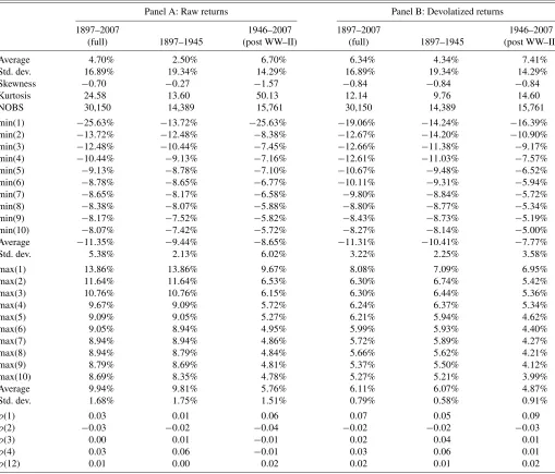
The focal point of Table2is daily raw returns (Panel A) and devolatized returns (Panel B) and their empirical attributes. To make comparisons meaningful, the devolatized series is stan-dardized to match the volatility of raw returns. Such an ap-proach merely scales the devolatized return distribution by a fixed constant. The point that needs to be emphasized here is that accounting for return volatility substantially reduces the kurtosis of the devolatized returns. The order of reduction is 50% over 1897–2007 sample period and 70% over the 1946– 2007 sample period.
Table2reveals an inherently puzzling empirical regularity of the stock markets with respect to price movements: the daily stock market crashes are harsh relative to stock market rallies. The largest daily percentage DJIA price decline of 25.63% (on October 19, 1987), for instance, is of substantially higher mag-nitude relative to the maximum daily percentage DJIA rise of 13.86% (on October 6, 1931). Over the 1897–2007 sample, the average across the ten largest crashes is −11.35% (cross-sectional standard deviation of 5.38%) compared to 9.94% (cross-sectional standard deviation of 1.68%) across the ten largest rallies. Another asymmetry exists between crashes and
rallies in the 1946–2007 sample with average across the ten largest crashes (rallies) being−8.65% (5.76%).
Furthermore, the post 1946 equity market is more resilient to external shocks: with the exception of the 1987 crash, the amplitude of crashes and rallies are markedly different between the pre and post 1946 stock markets. The largest 10 single-day rallies pre 1946 range between 8.35% and 13.86%, while the corresponding range of single-day rallies is 4.78% to 9.67% in the post 1946 sample. From the beginning of 1946 through the end of 2007, there are only 10 large downward movements be-yond 5%.
Even though the impact of devolatization is to generate a markedly lower kurtosis, the amplitude asymmetry between crashes and rallies is clearly detected in devolatized returns as well. Other than magnifying the dichotomy between the tails, the devolatized return distribution shares qualitatively similar features of crashes and rallies explicit in the raw return data. Furthermore, based on conventional criteria, the autocorrela-tions of raw returns and devolatized returns are negligible and do not exceed 0.06 and 0.09 in absolute value for raw and de-volatized returns, respectively.
Why are daily market price declines much larger in absolute value than daily price rises? The divergence between the inten-sities of crashes and rallies presents a challenge for theoretical models of market return dynamics. We will revisit this theme in the ensuing discussion.
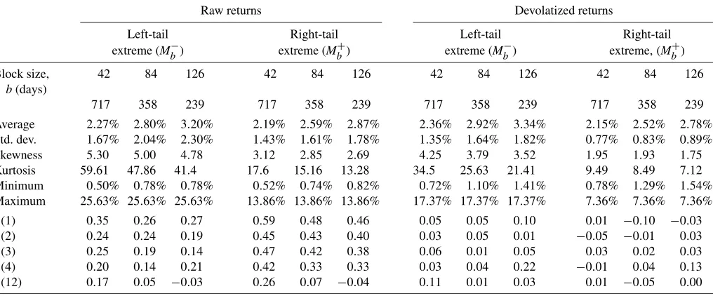
4.2 Comparative Behavior of ExtremesM−b andM+b
Even though in the real world there may be time-variation in the neck of the return distribution, we explore the hypothesis that if one looks away from the center of the empirical distribu-tion and puts aside small movements, it can be conjectured that tail movements are close to iid. That is, the operation of tak-ing maximum on daily movements over a block of observations focuses attention to the tails, and allows us to investigate large movements in either direction. There may be value in looking at the laws of tail movements as it exemplifies features that can be used to build more realistic models of local motion.
Thus, guided by our findings on the amplitude of daily crashes and rallies, we are prompted to ask: Is the comparative behavior of the left-tail unique? What time series evidence can be brought to bear on the behavior of extremes and tail events? To go to the heart of these questions using extreme value the-ory, we, henceforth, proxy jumps with daily return moves and consider a sequence of iid variables{z(i)}Ni=1. By dividing the entire dataset intonnonoverlapping subsamples and taking the maximum,M−(j)orM+(j), from every subsample, we end up with a sequence of maxima,{M−(j)}nj=1and{M+(j)}nj=1whose limit law is characterized by the Fisher–Tippett theorem.
With the view to balance concerns with respect to maxima obtained over shorter block sizes versus longer block sizes, we experimented with block size,b, of 42 days (2 months), 84 days
Table 2. Raw and devolatized Dow Jones industrial average daily returns
Panel A: Raw returns Panel B: Devolatized returns
1897–2007 1946–2007 1897–2007 1946–2007
(full) 1897–1945 (post WW–II) (full) 1897–1945 (post WW–II) Average 4.70% 2.50% 6.70% 6.34% 4.34% 7.41% Std. dev. 16.89% 19.34% 14.29% 16.89% 19.34% 14.29% Skewness −0.70 −0.27 −1.57 −0.84 −0.84 −0.84 Kurtosis 24.58 13.60 50.13 12.14 9.76 14.60
NOBS 30,150 14,389 15,761 30,150 14,389 15,761
min(1) −25.63% −13.72% −25.63% −19.06% −14.24% −16.39% min(2) −13.72% −12.48% −8.38% −12.67% −14.20% −10.90% min(3) −12.48% −10.44% −7.45% −12.66% −11.38% −9.17% min(4) −10.44% −9.13% −7.16% −12.61% −11.03% −7.57% min(5) −9.13% −8.78% −7.10% −10.67% −9.48% −6.52% min(6) −8.78% −8.65% −6.77% −10.11% −9.31% −5.94% min(7) −8.65% −8.17% −6.58% −9.80% −8.84% −5.72% min(8) −8.38% −8.07% −5.88% −8.80% −8.77% −5.34% min(9) −8.17% −7.52% −5.82% −8.43% −8.73% −5.19% min(10) −8.07% −7.42% −5.72% −8.27% −8.14% −5.00% Average −11.35% −9.44% −8.65% −11.31% −10.41% −7.77% Std. dev. 5.38% 2.13% 6.02% 3.22% 2.25% 3.58% max(1) 13.86% 13.86% 9.67% 8.08% 7.09% 6.95% max(2) 11.64% 11.64% 6.53% 6.30% 6.74% 5.42% max(3) 10.76% 10.76% 6.15% 6.30% 6.44% 5.36% max(4) 9.67% 9.09% 5.72% 6.24% 6.37% 5.34% max(5) 9.09% 9.05% 5.27% 6.21% 5.94% 4.62% max(6) 9.05% 8.94% 4.95% 5.99% 5.93% 4.40% max(7) 8.94% 8.94% 4.86% 5.72% 5.89% 4.27% max(8) 8.94% 8.79% 4.84% 5.66% 5.62% 4.21% max(9) 8.79% 8.69% 4.81% 5.37% 5.50% 4.12% max(10) 8.69% 8.35% 4.78% 5.27% 5.21% 3.99% Average 9.94% 9.81% 5.76% 6.11% 6.07% 4.87% Std. dev. 1.68% 1.75% 1.51% 0.79% 0.58% 0.91%
ρ(1) 0.03 0.01 0.06 0.07 0.05 0.09
ρ(2) −0.03 −0.02 −0.04 −0.02 −0.02 −0.03
ρ(3) 0.00 0.01 −0.01 0.02 0.04 0.01
ρ(4) 0.03 0.06 −0.01 0.03 0.06 0.01
ρ(12) 0.01 0.00 0.02 0.02 0.01 0.02
NOTE: Reported are average, standard deviation, skewness, kurtosis, minimum (calculated as the largest percentage daily price drop), and maximum (calculated as the largest percentage daily price rise). The average return and standard deviation are annualized by respectively scaling the daily counterparts by 252 and√252. The autocorrelation coefficient at lagjis denoted byρ(j). Here{min(j)}10j
=1({max(j)}10j=1) are the ordered largest negative (positive) daily moves. NOBS denotes the number of observations. The first trading day for
DJIA is January 2, 1897, and the last day is December 31, 2007 (111 years of daily data). Devolatized returns are calculated asXt/σt, where lnσ2t=1IIi−1
=0log((Xt−i)2), with an optimally chosenIset to 45 days. Devolatized returns are scaled to equalize the variance of raw returns and devolatized returns in each sample period.
(4 months), and 126 days (6 months) resulting innequal to 717, 358, and 239, respectively.
The results reported in Table3merit some remarks. First, an investor with a long (short) position in the DJIA can be expected to experience a maximum daily loss of 3.20% (2.87%) every six months. Second the series of left-tail extremes{M−(j)}nj=1
is far more volatile with kurtosis many times that of the right-tail extremes{M+(j)}nj=1. Third, in raw returns, the right-tail extremes are substantially more autocorrelated compared to the left-tail extremes and show slow decay even up to a longer lag. In other words, right-tail extremes have longer memories with large movements followed by movements of similar size (and the reverse), while left-tail extremes tend to be more idiosyn-cratic, which may reconcile why such events are traditionally difficult to hedge a priori. In contrast, both right-tail extremes
and left-tail extremes in devolatized returns show little evidence for autocorrelation.
Next, we apply the Kolmogorov–Smirnov statistic to test the null hypothesis that the left- and the right- tail events belong to the same distribution.
42 days 84 days 126 days Raw returns,p-value 0.46 0.09 0.11 Devolatized returns,p-value 0.00 0.00 0.00
The p-values of the Kolmogorov–Smirnov statistic reported above indicate that the null hypothesis cannot be rejected for raw returns, but is rejected on devolatized returns. In sum, ac-counting for time-varying return volatility in our
Table 3. Behavior of extremes,Mb−andMb+
Raw returns Devolatized returns
Left-tail Right-tail Left-tail Right-tail extreme (Mb−) extreme (Mb+) extreme (Mb−) extreme,(M+b) Block size, 42 84 126 42 84 126 42 84 126 42 84 126
b(days)
n 717 358 239 717 358 239 717 358 239 717 358 239 Average 2.27% 2.80% 3.20% 2.19% 2.59% 2.87% 2.36% 2.92% 3.34% 2.15% 2.52% 2.78% Std. dev. 1.67% 2.04% 2.30% 1.43% 1.61% 1.78% 1.35% 1.64% 1.82% 0.77% 0.83% 0.89% Skewness 5.30 5.00 4.78 3.12 2.85 2.69 4.25 3.79 3.52 1.95 1.93 1.75 Kurtosis 59.61 47.86 41.4 17.6 15.16 13.28 34.5 25.63 21.41 9.49 8.49 7.12 Minimum 0.50% 0.78% 0.78% 0.52% 0.74% 0.82% 0.72% 1.10% 1.41% 0.78% 1.29% 1.54% Maximum 25.63% 25.63% 25.63% 13.86% 13.86% 13.86% 17.37% 17.37% 17.37% 7.36% 7.36% 7.36%
ρ(1) 0.35 0.26 0.27 0.59 0.48 0.46 0.05 0.05 0.10 0.01 −0.10 −0.03
ρ(2) 0.24 0.24 0.19 0.45 0.43 0.40 0.03 0.05 0.01 −0.05 −0.01 0.03
ρ(3) 0.25 0.19 0.14 0.47 0.42 0.38 0.06 0.01 0.05 0.03 0.02 0.03
ρ(4) 0.20 0.14 0.21 0.42 0.33 0.33 0.03 0.04 0.22 −0.01 0.04 0.13
ρ(12) 0.17 0.05 −0.03 0.26 0.07 −0.04 0.11 0.01 0.03 0.01 −0.05 0.00
NOTE: For this exercise we fix a block sizebfor daily returns and set it equal to 42 days, 84 days, and 126 days. By dividing the entire dataset intonnonoverlapping subsamples of lengthband taking the maximum,M−(j)orM+(j), from every subsample, we obtain a series of maxima,{M−(j)}n
j=1and{M+(j)}nj=1. Reported are the average, standard deviation,
skewness, kurtosis, minimum, and maximum of the respective series. The autocorrelation coefficient at lagjis denoted byρ(j).
tion procedure accentuates the distinction between the left- and right-tails.
4.3 Historical Probabilities of Crashes and Rallies
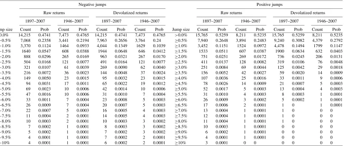
In view of our goal to examine whether the observed ar-rival rates of negative and positive price jumps conform to vari-ous Lévy measures, we decompose daily price fluctuations into their positive and negative constituents. We subdivide the uni-verse of possible negative jump sizes into 21 classifications ranging from<0%,≤−0.5%,≤−1.0%, . . . , <−10% (in incre-ments of−0.5%) and the same for positive return jumps. The zero return observations are excluded and hence the total num-ber of observations drops to 29,980.
Concentrate on the heading marked “Negative Jumps” in Ta-ble4. For this jump classification, we calculate the number of instances a stock price jump of size less than or equal to, say, 5% has occurred. Record this statistic as “Count.” Then, the
probabilityof the stock price jump of the same size is “Count” divided by the universe of all jump sizes. We record this statistic under the heading “Prob.”
Tables4and5offer a coherent picture of the arrival rate of crashes to rallies and also their historical probabilities of occur-rence. The main empirical findings are as follows.
First, the probability of a positive jump in the DJIA of all sizes, whether raw or devolatized, surpasses the negative coun-terpart by about 5%. For example, over the entire 111 years, the market declined on 14,215 days and rose on 15,765 days. This outcome translates into a 47.41% probability of a decline and a 52.59% of a stock market rise. The decline probability is 47.65% during the 1946–1997 DJIA period.
Second, rally and crash probabilities of the same magnitude exhibit pronounced asymmetries in both raw returns and de-volatized returns. Considering the full period, as often as 321 (251) times, the raw DJIA declined (rose) more than 3%. More
fundamentally, on any given day, the market declined (rose) by more than 5% on 69 (52) occasions. Overall, this amounts to a 0.23% probability for a daily decline of 5% or higher, and 0.17% for a surge of 5% or more. Along the same lines, a daily catastrophic drop of 10% or higher has been observed four times in the entire period while surges exceeding this magnitude have occurred three times. The higher probability of crashes poses a puzzle: why have equity markets experienced a higher number of crashes than rallies?
Third, crash and rally frequencies differ radically depending on whether one is considering the post or pre 1946 stock mar-kets. Out of the total 69 crashes in the DJIA of 5% or higher, 59 crashes (or 86%) were confined to pre 1946 period, and only 10 to the post 1946 period. Out of 52 rallies, only 5 are attributable to the post 1946 period. Not only has the probability of a crash decreased dramatically in the post 1946 period, the probability of a rally has also declined.
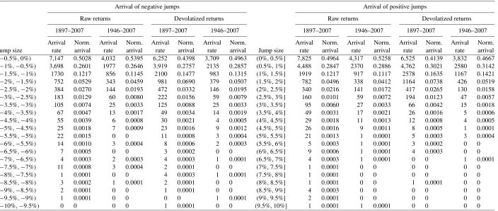
Fourth, we can extract thejump arrival ratesand normalized jump arrival rates directly from Table4. We report these under “Arrival rate” and “Norm. arrival” in Table5. The normalized arrival rate of, e.g., a negative jump size−2% to−2.5% can be recovered by counting all jumps in this range and then dividing the count by the number of negative jumps of all sizes.
Based on Table 5, several points can be established. One, jumps of small magnitude have strictly higher arrival rates than jumps of larger magnitude. This pattern is particularly clear in devolatized returns. Two, during the post 1946 sample, the majority of the jumps (positive or negative) are of relatively smaller magnitude. For example, 80.41% (81.44%) of the neg-ative (positive) jumps are concentrated between 0 to−1%. The arrival rates of positive and negative jumps are also sparse be-yond 10%. Three, there does not appear to be any association between the arrival rates of positive and negative jumps for any jump size.
Madan,
and
P
ana
y
oto
v:
Deducing
the
Implications
of
J
ump
Models
389
Table 4. Probabilities of stock market declines and rises of all sizes
Negative jumps Positive jumps
Raw returns Devolatized returns Raw returns Devolatized returns 1897–2007 1946–2007 1897–2007 1946–2007 1897–2007 1946–2007 1897–2007 1946–2007 Jump size Count Prob Count Prob Count Prob Count Prob Jump size Count Prob Count Prob Count Prob Count Prob
<0.0% 14,215 0.4741 7,473 0.4765 14,215 0.4741 7,473 0.4765 >0.0% 15,765 0.5259 8,211 0.5235 15,765 0.5259 8,211 0.5235
≤−0.5% 7,068 0.2358 3,441 0.2194 7,963 0.2656 3,764 0.24 ≥0.5% 7,940 0.2648 3,894 0.2483 9,240 0.3082 4,379 0.2792
≤−1.0% 3,370 0.1124 1464 0.0933 4,044 0.1349 1629 0.1039 ≥1.0% 3,452 0.1151 1524 0.0972 4,478 0.1494 1799 0.1147
≤−1.5% 1640 0.0547 608 0.0388 1944 0.0648 646 0.0412 ≥1.5% 1533 0.0511 607 0.0387 1900 0.0634 632 0.0403
≤−2.0% 888 0.0296 265 0.0169 963 0.0321 267 0.0170 ≥2.0% 751 0.0251 269 0.0172 736 0.0245 206 0.0131
≤−2.5% 504 0.0168 121 0.0077 491 0.0164 121 0.0077 ≥2.5% 411 0.0137 128 0.0082 319 0.0106 76 0.0048
≤−3.0% 321 0.0107 61 0.0039 269 0.0090 62 0.0040 ≥3.0% 251 0.0084 69 0.0044 125 0.0042 29 0.0018
≤−3.5% 216 0.0072 36 0.0023 144 0.0048 37 0.0024 ≥3.5% 156 0.0052 42 0.0027 59 0.0020 14 0.0009
≤−4.0% 149 0.0050 23 0.0015 95 0.0032 23 0.0015 ≥4.0% 107 0.0036 25 0.0016 33 0.0011 9 0.0006
≤−4.5% 94 0.0031 17 0.0011 65 0.0022 19 0.0012 ≥4.5% 78 0.0026 14 0.0009 21 0.0007 5 0.0003
≤−5.0% 69 0.0023 10 0.0006 42 0.0014 10 0.0006 ≥5.0% 52 0.0017 5 0.0003 13 0.0004 4 0.0003
≤−5.5% 47 0.0016 10 0.0006 31 0.0010 7 0.0004 ≥5.5% 31 0.0010 4 0.0003 8 0.0003 1 0.0001
≤−6.0% 33 0.0011 7 0.0004 23 0.0008 5 0.0003 ≥6.0% 26 0.0009 3 0.0002 5 0.0002 1 0.0001
≤−6.5% 26 0.0009 7 0.0004 20 0.0007 5 0.0003 ≥6.5% 17 0.0006 2 0.0001 1 0 1 0.0001
≤−7.0% 22 0.0007 5 0.0003 16 0.0005 4 0.0003 ≥7.0% 13 0.0004 1 0.0001 1 0 0 0
≤−7.5% 11 0.0004 2 0.0001 14 0.0005 4 0.0003 ≥7.5% 12 0.0004 1 0.0001 1 0 0 0
≤−8.0% 10 0.0003 2 0.0001 10 0.0003 3 0.0002 ≥8.0% 11 0.0004 1 0.0001 1 0 0 0
≤−8.5% 7 0.0002 1 0.0001 8 0.0003 3 0.0002 ≥8.5% 10 0.0003 1 0.0001 0 0 0 0
≤−9.0% 5 0.0002 1 0.0001 7 0.0002 3 0.0002 ≥9.0% 6 0.0002 1 0.0001 0 0 0 0
≤−9.5% 4 0.0001 1 0.0001 7 0.0002 2 0.0001 ≥9.5% 4 0.0001 1 0.0001 0 0 0 0
≤−10% 4 0.0001 1 0.0001 6 0.0002 2 0.0001 ≥10% 3 0.0001 0 0 0 0 0 0
NOTE: Each for raw returns and devolatized returns, the daily returns are initially divided into negative movements and positive movements. Tracking the negative and positive movements separately, we compute the distribution of negative movements as<0.0%,≤−0.50%, . . . ,≤−10.0% and for positive movements as>0.0%,≥0.5%, . . . ,≥10.0%. In what is reported, the probability (denoted “Prob”) of a stock market decline or a rise in certain size range is then computed by normalizing the number of moves in this range (denoted “Count”) by the total number of trading days in the respective sample. The notation of NOBS is the number of trading days. The number of observations in the 1897–2007 (1946–2007) sample period is 29,980 (15,684), whereby days with no price change are excluded.
Jour
nal
of
Business
&
Economic
Statistics
,
J
uly
2010
Table 5. Lévy measure and the arrival rates of negative and positive jumps
Arrival of negative jumps Arrival of positive jumps
Raw returns Devolatized returns Raw returns Devolatized returns 1897–2007 1946–2007 1897–2007 1946–2007 1897–2007 1946–2007 1897–2007 1946–2007 Arrival Norm. Arrival Norm. Arrival Norm. Arrival Norm. Arrival Norm. Arrival Norm. Arrival Norm. Arrival Norm. Jump size rate arrival rate arrival rate arrival rate arrival Jump size rate arrival rate arrival rate arrival rate arrival
[−0.5%,0%) 7,147 0.5028 4,032 0.5395 6,252 0.4398 3,709 0.4963 (0%, 0.5%] 7,825 0.4964 4,317 0.5258 6,525 0.4139 3,832 0.4667
[−1%,−0.5%) 3,698 0.2601 1977 0.2646 3,919 0.2757 2135 0.2857 (0.5%, 1%] 4,488 0.2847 2370 0.2886 4,762 0.3021 2580 0.3142
[−1.5%,−1%) 1730 0.1217 856 0.1145 2100 0.1477 983 0.1315 (1%, 1.5%] 1919 0.1217 917 0.1117 2578 0.1635 1167 0.1421
[−2%,−1.5%) 752 0.0529 343 0.0459 981 0.0690 379 0.0507 (1.5%, 2%] 782 0.0496 338 0.0412 1164 0.0738 426 0.0519
[−2.5%,−2%) 384 0.0270 144 0.0193 472 0.0332 146 0.0195 (2%, 2.5%] 340 0.0216 141 0.0172 417 0.0265 130 0.0158
[−3%,−2.5%) 183 0.0129 60 0.0080 222 0.0156 59 0.0079 (2.5%, 3%] 160 0.0101 59 0.0072 194 0.0123 47 0.0057
[−3.5%,−3%) 105 0.0074 25 0.0033 125 0.0088 25 0.0033 (3%, 3.5%] 95 0.0060 27 0.0033 66 0.0042 15 0.0018
[−4%,−3.5%) 67 0.0047 13 0.0017 49 0.0034 14 0.0019 (3.5%, 4%] 49 0.0031 17 0.0021 26 0.0016 5 0.0006
[−4.5%,−4%) 55 0.0039 6 0.0008 30 0.0021 4 0.0005 (4%, 4.5%] 29 0.0018 11 0.0013 12 0.0008 4 0.0005
[−5%,−4.5%) 25 0.0018 7 0.0009 23 0.0016 9 0.0012 (4.5%, 5%] 26 0.0016 9 0.0011 8 0.0005 1 0.0001
[−5.5%,−5%) 22 0.0015 0 0 11 0.0008 3 0.0004 (5%, 5.5%] 21 0.0013 1 0.0001 5 0.0003 3 0.0004
[−6%,−5.5%) 14 0.0010 3 0.0004 8 0.0006 2 0.0003 (5.5%, 6%] 5 0.0003 1 0.0001 3 0.0002 0 0
[−6.5%,−6%) 7 0.0005 0 0 3 0.0002 0 0 (6%, 6.5%] 9 0.0006 1 0.0001 4 0.0003 0 0
[−7%,−6.5%) 4 0.0003 2 0.0003 4 0.0003 1 0.0001 (6.5%, 7%] 4 0.0003 1 0.0001 0 0 1 0.0001
[−7.5%,−7%) 11 0.0008 3 0.0004 2 0.0001 0 0 (7%, 7.5%] 1 0.0001 0 0 0 0 0 0
[−8%,−7.5%) 1 0.0001 0 0 4 0.0003 1 0.0001 (7.5%, 8%] 1 0.0001 0 0 0 0 0 0
[−8.5%,−8%) 3 0.0002 1 0.0001 2 0.0001 0 0 (8%, 8.5%] 1 0.0001 0 0 1 0.0001 0 0
[−9%,−8.5%) 2 0.0001 0 0 1 0.0001 0 0 (8.5%, 9%] 4 0.0003 0 0 0 0 0 0
[−9.5%,−9%) 1 0.0001 0 0 0 0 1 0.0001 (9%, 9.5%] 2 0.0001 0 0 0 0 0 0
[−10%,−9.5%) 0 0 0 0 1 0.0001 0 0 (9.5%, 10%] 1 0.0001 1 0.0001 0 0 0 0
NOTE: In order to conform with the definition of Lévy measure for jump sizez<0 andz>0, the daily returns are initially divided into negative movements and positive movements. Forz<0 we compute the frequency of movements in 21 buckets as [−0.5%,0%),[−1%,−0.5%), . . . ,[−10%,−9.5%), and forz>0 also in 21 buckets as(0,0.5%], (0.50%,1%], . . . ,[9.5%,10.0%). Respectively for the stock market declines (rises), the empirical “Arrival rate” is obtained by computing the number of negative (positive) jumps in each size bucket. On the other hand, “Norm. arrival” is the arrival rate divided by the total number of negative (positive) jumps in the respective period.
5. DISENTANGLING THE STRUCTURE OF JUMPS
Since every jump model can be characterized by its Lévy measure, we can ask the following important question using de-volatized returns: Which Lévy measure, and accordingly, which theoretical model best matches the pattern of jump arrival rates observed in the stock market?
To describe the rationale for the empirical specifications and the associated testable restrictions, consider the Lévy measures
(z)for the jump models in Equations (13), (16), (17), and (18). Since Lévy measures link arrival rate of jumps to jump size, we can regress ln(z)on model-specific functions of the jump sizezand determine the internal consistency of the result-ing regression coefficients. In our implementation, we surrogate
(z)by the arrival rate of jumps as shown in Table5, andzby the jump size interval midpoint.
Germane to the jump model in Equation (13) is the empirical specification in log-form of the type
ln[z] =0+1|z|1z<0+2z1z>0+3ln(|z|), (30) which generates the testable restrictions 1= −λ−<0 and
2= −λ+<0. Equation (30) is amenable to casting 3=
−(1 +ξ ), where ξ corresponds to the exponent in Equa-tion (18). The wider interest inξ stems from the fact that it governs the departure from Equation (13), and hence3 regu-lates the nature of small activity. If inferences regarding small
moves are to be drawn based on estimated3, then small move-ments should not be discarded since they are an integral part of the Lévy measure.
Estimated magnitude of3is key to validating finite activity (i.e., ξ <0 and hence 3>−1), infinite activity (i.e., ξ >0 and hence3<−1), or infinite variation (i.e.,ξ >1 and hence
3<−2). The exponent on the Lévy measure in Equation (13) is exactly unity whenξ=0, a testable hypothesis.
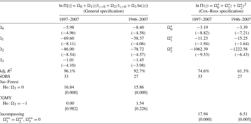
The results shown in Table6confirm the plausibility of the jump model in Equation (13) in explaining the jump structure in market returns observed since 1897. First, in line with theory,
1<0 and2<0, which supports the completely monotone property of the Lévy measure. Second, the estimated coeffi-cients implyλ−= −1=69.60,λ+= −2=86.00, and cru-cially λ−< λ+. Statistical significance of 1 and 2 is not a concern as the minimum absolute t-statistic is 4.06. More-over, it is the distinction betweenλ−andλ+that epitomizes the asymmetry between the arrival rate of downward jumps versus positive jumps. Often this feature is difficult to identify in raw returns, but devolatization has sharpened return asymmetries embedded in the Lévy measures (see also Barndorff-Nielsen
1998).
Returning to 3, we infer that it is −1.01 (t-statistic of
−4.10) and −1.45 (t-statistic of −3.98), respectively, over 1897–2007 and 1946–2007. Furthermore the null hypothesis
3= −1 is not rejected. The conventional F-test statistic for
Table 6. Testing the restrictions on the Lévy measures based on devolatized data
ln[z] =0+1|z|1z<0+2z1z>0+3ln(|z|) ln(z)=∗0+∗1z+∗2z2
(General specification) (Cox–Ross specification) 1897–2007 1946–2007 1897–2007 1946–2007
0 −5.98 −8.40 ∗0 −3.19 −3.39
(−4.96) (−4.58) (−8.82) (−7.21)
1 −69.60 −58.37 ∗1 −11.23 −15.25
(−8.11) (−4.06) (−1.94) (−1.64)
2 −86.00 −78.72 ∗2 −1062.39 −1222.58
(−8.54) (−4.57) (−9.53) (−6.43)
3 −1.01 −1.45
(−4.10) (−3.98)
Adj.R2 96.1% 92.7% 74.6% 61.3%
NOBS 33 27 33 27
Das–Foresi
Ho :3=0 16.84 15.86
{0.000} {0.000}
CGMY
Ho :3= −1 0.00 1.54
{0.982} {0.226}
Encompassing 17.94 6.51
∗∗1 =∗∗2 ,∗∗3 =0 {0.000} {0.005}
NOTE: In the regression analysis, the log of the Lévy measure, ln(z)is the dependent variable where(z)is surrogated by the arrival rate of jumps andzby the jump size interval midpoint, as shown in Table5. Thet-statistics are reported in parenthesis. We investigate the empirical specification,
ln[z] =0+1|z|1z<0+2z1z>0+3ln(|z|).
First, if3=0, we get the Lévy measure in Das and Foresi (1996). Second, if3= −1, we cannot reject the jump model in Equations (5)–(7) that gives rise to the Lévy measure
in Equation (13). The parameter transformation are0= −ln(κ),1= −λ−<0,2= −λ+<0, and3= −(1+ξ ). The null hypothesis are tested using the standardF-test with
p-value in curly brackets. For the Cox and Ross (1976) model, we examine ln(z)=∗0+∗1z+∗2z2. The model imposes the testable restriction that the log Lévy measure is quadratic in the jump size with the sign of∗
1being the sign ofμJ, and∗2<0. The comparison between the pure-jump model and the Cox–Ross model is examined in the row “Encompassing,”
which represents an artificial encompassing specification of the type:
ln[z] =0+1∗∗|z|1z<0+∗∗2 z1z>0+∗∗3 ln(|z|)+∗∗4 z2.
The joint restriction is∗∗1 =∗∗2 , and∗∗3 =0. Reported is the value of theF-statistic along with thep-value in curly brackets.
this hypothesis does not exceed 1.54 (p-value 0.226). Based on this test,ξ is indistinguishable from zero.
An advantage of adopting specification in Equation (30) is that it also nests the log Lévy measure for the Das–Foresi jump-model. TheF-test reported in Table6 examines the exclusion restriction3=0. Thep-values indicate an overwhelming re-jection of the Das and Foresi (1996) and Kou (2002) jump mod-els.
How does the quadratic arrival rate model of Cox and Ross (1976) fare with respect to the purely discontinuous counterpart in capturing jump arrival rates? The model imposes the testable restriction that the log Lévy measure is quadratic in the jump size with the sign of∗1being the sign ofμJand∗2<0: meters of the jump distribution are unreasonable, based on what is known from Bakshi, Cao, and Chen (2000), Bates (2000), and Eraker, Johannes, and Polson (2003). To examine model failure from a different angle, we take an artificial encom-passing regression ln[z] =∗∗0 +∗∗1 |z|1z<0+∗∗2 z1z>0+
∗∗3 ln(|z|)+∗∗4 z2and test∗∗1 =∗∗2 and∗∗3 =0. The re-ported p-value indicates the inadequacy of the Cox and Ross (1976) model.
Overall, these results support the view that the structure of large movements has a fatter left-tail relative to the Gaussian distribution of jump sizes. Thus, the generalized LM in Equa-tion (13) may be needed for a better performing theory of stock market in the tails.
We should emphasize that the results in Table6should not be interpreted as an exact estimation of the Lévy measure. Suppose one generated (daily) returns from the geometric Brownian mo-tion model and then binned them according to size as done in Table5. At an empirical level the regression of the frequency of movements on size is valid even though there is no Lévy mea-sure for a geometric Brownian motion (the path is continuous). This observation bears analogy with the fact that a Lévy mea-sure of a process (when it exists), is the theoretical limit of the density divided by a small time intervaltas t→0, while at the same time this limit can be estimated even for processes with no Lévy measure. Therefore, Table6only presents a pos-sibly crude attempt to differentiate the tail behavior across mod-els. To rigorously extract the Lévy measure, one must estimate the structural parameters (say,σ, θ, κ) through maximum like-lihood of the return density and then recover the Lévy measure throughλ−andλ+, a task we turn to later.
6. DEDUCING THE LIMIT LAWS OF EXTREMES AND THE THICKNESS OF TAILS
Still three questions remain unanswered. First, are extreme fluctuations constructed from devolatized returns consistent with Fréchet or Weibull limit laws? Second, if a large scale sim-ulation is performed to approximaten→ +∞on the pure-jump
dynamics postulated in Equations (5) to (7), which limit law is supported? Each metric imposes a distinct barrier on the purely discontinuous price dynamics and the tail probability model. Finally, is the right-tail thinner than the left-tail based on the estimate of the tail-indexα?
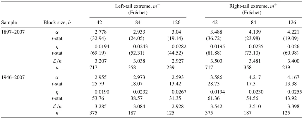
6.1 Limit Laws of Left-Tail Event Extremes and Right-Tail Event Extremes
To answer the first question, we fix, as before, the block size to 42 days, 84 days, and 126 days. Thus, we have a set of six block maximas{m−(j)}nj=1and{m+(j)}nj=1for devolatized re-turns, wherem−=exp(M−)−1 andm+=exp(M+)−1. Then, in the spirit of Pesaran and Deaton (1978), the examination of the Weibull versus Fréchet limit laws can be conducted by max-imizing the log-likelihood function, where the functional form of the Fréchet density, denoted F[·], and the Weibull density, denoted W[·], are as pre-sented in Equations (23) and (24). In the artificially nested log-likelihood function in Equation (32), the null of Weibull limit law versus Fréchet is equivalent to testing whetherŴ=0 and is a hypothesis on the boundary.
When data are uncertain about the parametric form of the underlying density, our maximum likelihood estimations reveal that Weibull is being rejected in favor of the Fréchet for both
m− orm+. In particular, the estimatedŴis virtually unity and the null hypothesisŴ=0 is rejected. Thus, the goodness-of-fit diagnostic is suggesting the Fréchet distribution as the limit law for both the left-tail and right-tail events.
Fréchet distribution asserts a power law tail behavior, that is, limm→∞ F[m] →m1α+α, and, hence, heavy tailed extremes. It
must be appreciated that the tail indexα is directly linked to the tail heaviness and the number of bounded moments of the extremes (Feller1971), with 1+α=supj>1
mj F[m]dm<
∞.
The fundamental observation that can be garnered from Ta-ble7is that the maximum likelihood estimations are stipulat-ing that the tail-index,α, is substantially different for left-tail extremesm− versus right-tail extremes m+. For negative ex-tremes,αis in the range of 2.593 and 3.040, while for positive extremes,α is in the range of 3.448 to 4.221. Thet-statistics reported in parenthesis are large.
Consider block size of 126 days over 1897–2007. The entry ofα=3.04 implies finite moments up to order 4 for the dis-tribution ofm− whereas the entry ofα=4.221 implies finite moments up to order 5 for the distribution ofm+. Essentially the distribution of right-tail events has thinner tail and gravi-tates to zero at a faster rate. The distribution of left-tail events has an even heavier tail in the post 1946 period. Longin (1996) arrived at the Fréchet limit law for the S&P 500 index. The work here differs from Longin (1996) and a related study by Jansen and Vries (1991) in two ways. First, we develop and empiri-cally examine a model of stock market extremes, their arrival