Full Terms & Conditions of access and use can be found at
http://www.tandfonline.com/action/journalInformation?journalCode=ubes20
Download by: [Universitas Maritim Raja Ali Haji] Date: 12 January 2016, At: 00:15
Journal of Business & Economic Statistics
ISSN: 0735-0015 (Print) 1537-2707 (Online) Journal homepage: http://www.tandfonline.com/loi/ubes20
Estimating Panel Models With Internal and
External Habit Formation
George M. Korniotis
To cite this article: George M. Korniotis (2010) Estimating Panel Models With Internal and
External Habit Formation, Journal of Business & Economic Statistics, 28:1, 145-158, DOI: 10.1198/jbes.2009.08041
To link to this article: http://dx.doi.org/10.1198/jbes.2009.08041
Published online: 01 Jan 2012.
Submit your article to this journal
Article views: 196
View related articles
Estimating Panel Models With Internal
and External Habit Formation
George M. K
ORNIOTISBoard of Governors of the Federal Reserve System, Division of Research and Statistics, Risk Analysis Section (Mail Stop 91), 20th Street and Constitution Avenue NW, Washington, DC 20551 (George.M.Korniotis@frb.gov)
A new bias-corrected estimator is developed for dynamic panel model with both fixed and spatial effects. The estimator is asymptotically unbiased, normally distributed, and it has good finite sample properties (low finite sample bias and root mean squared error). Applying the estimator to annual consumption data for the continental U.S. states shows that state consumption growth is not significantly affected by its own (lagged) consumption growth. However, it is affected by lagged consumption growth of nearby states. These results support external habit formation model, which have been used to explain the behavior of U.S. stock returns.
KEY WORDS: Asset pricing; Bias correction; Instrumental variables; Spatial and dynamic effects; U.S. state consumption.
1. INTRODUCTION
This paper introduces a new bias-corrected estimator for dy-namic panel models with fixed and spatial effects to test for habit formation at the aggregate level. Testing for habit for-mation is important because consumption-based asset pricing models with habits are a leading class of models that explain as-set pricing phenomena (Constantinides2002). In these models, the welfare of the consumer depends on the difference between actual consumption and a habit level of consumption. The habit is a time-varying subsistence level, and it typically takes one of two forms. For models in which the determinants of the habit are internal to the consumer (internal habit), the consumers’ consumption habits are influenced by own past consumption (Constantinides1990; Ferson and Constantinides1991; Ferson and Harvey1992; Dynan2000; Fuhrer2000). For models in which the determinants of the habit are external to the consumer (external habit), consumers’ consumption habits are influenced by the consumption decisions ofotherconsumers (Abel1990; Gali1994; Campbell and Cochrane1999; Wachter2006). Even though internal and external habits are widely used, there are only a couple of studies estimating models that include both of them (Grishchenko2007; Ravina2007).
Since little is known about the relative importance of internal and external habits, I test for their significance by estimating Euler equations with data for the 48 continental U.S. states. As in Ferson and Constantinides (1991), the measure of the internal component of the habit is past own consumption. As in Abel (1990), the measure of the external component of the habit is a weighted average of past consumption growth rates of other cross-sectional units; this type of external habit is called “catching up with the Joneses.” The external habit of a state is a spatially lagged dependent variable because it is given by consumption growth rates of other states spatially located in the same national economy. The Euler equation of the eco-nomic model with both types of habit formation produces a dynamic panel regression in which the dependent variable is the consumption growth rate of each U.S. state. The regression includes fixed effects to allow for heterogeneous rates of con-sumption growth across the U.S. states. The regression involves
a time-lagged dependent variable (the internal-habit measure) and a spatially lagged dependent variable (the external-habit measure). The regression also contains the contemporaneous return of the one-month U.S. Treasury bill (the endogenous re-gressor).
The existing literature provides little guidance on estimat-ing panel regression models with habit variables and endoge-nous regressors. I therefore introduce a new estimator, which extends the work of Hahn and Kuersteiner (2002) on estimating dynamic panel models with the least-squares dummy variable (LSDV) estimator. My extension, which allows for spatial ef-fects and endogenous control variables, is a hybrid of the LSDV and the instrumental variable estimator of Anderson and Hsiao (1982). Like Hahn and Kuersteiner (2002), I rescale (de-mean) the data to eliminate the fixed effects from the estimation, and, like Anderson and Hsiao (1982), I instrument the endogenous control variables. I show that the hybrid estimator is asymp-totically biased. I therefore use its asymptotic bias to define a bicorrected estimator that is asymptotically unbiased and as-ymptotically normal.
In practice, the bias-corrected estimator might be preferred to a pure instrumental variable (IV) estimator because it only instruments the explanatory variables whereas an IV estima-tor has to also instrument the time-lagged and spatially lagged dependent variables. Consequently, the IV might be more ex-posed to weak instrument biases compared to the bias-corrected estimator. For example, see Hahn, Hausman, and Kuersteiner (2002).
Moreover, using Monte Carlo simulations, I find that the bias-corrected estimator compares favorably to a pure IV-type estimator. First, I find that the bias-corrected estimator has low finite-sample bias and low standard deviation. It also has a smaller root mean squared error than the pure IV estima-tor of Anderson and Hsiao (1982). Second, I find that in the presence of measurement error, the finite-sample bias of
© 2010American Statistical Association Journal of Business & Economic Statistics January 2010, Vol. 28, No. 1 DOI:10.1198/jbes.2009.08041
145
the bias-corrected estimator increases. The estimator however, maintains a low root mean squared error, and again has a lower standard deviation than the pure IV estimator.
I apply the bias-corrected estimator to test for habit forma-tion. Like most studies in the consumption-based asset pric-ing literature, I test for habit formation at the aggregate level. However, instead of using national data, I use annual data for the 48 continental U.S. states for the period 1966–1998. State-level data have important advantages when testing for habit for-mation. Specifically, even though state-level data are aggregate data, they exhibit considerable cross-sectional variation. Thus, for each state, I can define measures of external-habit formation that areindependentof internal-habit measures. For instance, if I am considering New Jersey, an external-habit measure can be the average of past consumption choices of states other than New Jersey, and a measure for the internal component of the habit is the past consumption level of New Jersey itself. This clear distinction between the two habit measures, which is lost when using national data, provides a powerful way to determine the type of habit best supported by the data.
In the empirical application, I measure internal-habit forma-tion by own past consumpforma-tion. I also consider various external-habit measures that exclude own consumption (Case 1991; Hernández-Murillo 2003; Ravina2007). The estimation finds supporting evidence for external-habit formation and provides only weak evidence of internal-habit formation. In particular, I find that the closer two states are, the more they affect each other, a result consistent with existing work (Case1991; Rav-ina2007). I also find suggestive evidence that states with popu-lation that predominantly lives in urban centers affect the con-sumption of other states the most. This last finding indicates that consumption trends might originate from urban centers.
Beyond testing for habit formation, the bias-corrected esti-mator is of practical relevance to a wide range of studies, such as country comparisons (Islam1995; Lee, Pesaran, and Smith 1998) and microeconomic studies using synthetic cohort data. Therefore, in Section 2, I present the panel model in general terms. In Section3, I define the bias-corrected estimator and its asymptotic properties. In Section4, I collect all the results re-lated to testing for habit formation at the U.S. state level, and in Section5, I present the results of a simulation exercise. The set-up of the simulation is based on the empirical results in Sec-tion4. In Section6, I conclude the discussion.
2. ECONOMETRIC MODEL
This paper introduces a procedure for estimating linear mod-els that includes fixed effects, a time-lagged dependent variable, and a spatially lagged dependent variable
Yit=π1Yi,t−1+ρ1 N
j=1
wijYj,t−1+Xitλ+ci+ηit,
i= [1, . . . ,N],t= [1, . . . ,T], (1)
where Yit is the dependent variable for cross-sectional unit i at time t. [Korniotis (2007) provides a generalization of the model withm1 time-lagged dependent variables, andm2 spa-tially lagged dependent variables.] The timing convention is that the available data for estimation is from t=0 to t=T.
Like Hahn and Kuersteiner (2002), the observation of the de-pendent variable att=0,Yi0, represents the initial condition of Yit, and is taken to be nonstochastic and known to the econo-metrician. The random variable ηit is an iid error term with zero mean and varianceση2. The constantci is the fixed effect of cross-sectional unitithat absorbs time-invariant characteris-tics ofiinfluencing the dependent variable. The vectorXit is a 1×Kvector of endogenous control variables (see Condition3 below for additional assumptions onXit). TheK×1 vectorλ includes the parameters related toXit. The set of control vari-ables can include contemporaneous and time-lagged values of Xit. Henceforth, matrices and vectors are in boldface font.
The weight wij measures the importance of Yj,t−1 on Yit. The weights are observed quantities, which are known to the econometrician, and they are therefore exogenous. Because the spatial lag,Nj=1wijYj,t−1, is a weighted average of past con-sumption choices of other cross-sectional units, it is the mea-sure of the catching-up habit. The weightswij are organized in theN×NmatrixWcalled the spatial matrix. The structure of Wis explained in Condition2below.
The presence of the fixed effects allows for nonparametric estimation of the time-invariant differences between the cross-sectional units. I choose the fixed effects model, over the ran-dom effects one, because it is more appropriate for models with habit formation. The economic model in Section4reveals that the fixed effects are related to state-specific discount rates. Since the state-specific discount rates depend on state character-istics (e.g., demographics), I cannot treat them as independent realization of a random shock, which is the assumption made in random effects models (e.g., Hausman1978). For similar rea-sons, Asdrubali, Sorensen, and Yosha (1996) and Ostergaard, Sorensen, and Yosha (2002) use the fixed effects specifica-tion when estimating panel models with state-level consump-tion data.
The econometric model (1) is different from the model in Hahn and Kuersteiner (2002) in two ways: It allows for en-dogenous control variables, and it includes the spatially lagged dependent variableNj=1wijYj,t−1. Moreover, the econometric model (1) operates under three conditions, which are presented next.
Condition 1. 1(1): The error termηit is iid acrossN andT. All the moments ofηitexist andE|ηit|2+ζ <∞for someζ >0 and alli andt. 1(2): The limit ofN/T exists (asN,T → ∞) and it is bounded between 0 and∞, that is, lim(N/T)=k, 0< k<∞. 1(3):|ρ1| + |π1|<1. 1(4): maxi|Yi0|2=O(
√
N). 1(5): maxi|ci|ζ =O(1),ζ >0.
Remark 1. Condition1(1) does not allow any cross-sectional or time correlations in the error term. Because the scope of model (1) is to estimate any time correlations (through time-lagged dependent variables) and any spatial correlations (through spatially lagged dependent variables), it is convenient to purge such effects from the error term. Among others, panel models with cross-sectional dependence in the error term are investigated in Conley (1999) and Phillips and Sul (2003).
Remark 2. Condition1(2) assumes thatT andN grow at a finite rate, which is in line with the asymptotic analysis in Hahn and Kuersteiner (2002).
Remark 3. Condition1(3) is a stationarity assumption. Con-ditions1(4) and1(5) control the behavior of the initial condi-tionsY0and the fixed effects, respectively.
Condition 2 (Spatial matrix). The matrix W is an N ×N matrix with wij being the element on its ith row and jth col-umn. 2(1):Wis a real nonnegative matrix, that iswij≥0 for alliandj. 2(2): All the diagonal elements ofWare zero, that iswii =0 for all i. 2(3): The rows ofW sum to one, that is
N
j=1wij=1 for alli. 2(4): The maximum column sum ofWis kc, andkcis finite and strictly less thank0= [(|π1| + |ρ1|)−1− |π1|]/|ρ1|. 2(5): AsN→ ∞,Wmaintains the above properties. Remark 4. Condition 2(1) holds for all spatial matrices. If wij>0, then unitj affects unit i. If wij=0, then unit j does not affecti. Condition2(2) is a normalization, which implies thatidoes not affect itself. Condition2(3) implies that spatial variables, likeNj=1wijYj,t−1, are weighted averages.
Remark 5. Conditions2(3) and 2(4) restrict the degree of cross-sectional correlation between the units. Note that in vir-tually all large sample theory one has to restrict the degree of permissible correlations. For example, see Kapoor, Kelejian, and Prucha (2007, assumption 4). They also ensure that W is uniformly bounded in the sense that the maximum rowsum
N tice it is very unlikely that it will be binding. For example, in the empirical application in Section4, across the various spa-tial matrices I consider, the largest value forkcis 2.49, and the smallest value fork0 is 32. The specific value ofk0is chosen for technical reasons explained in Korniotis (2007).
Remark 7. Under Condition2, the matrixWdoes not have to be symmetric. In fact, because the rows ofWsum to one, it is unlikely thatwijwill equal towji. Moreover, Condition2does not preclude cases wherewij>0 andwji=0. In this case,jis the leader and it affects, but it is not affected byi, the follower.
Condition 3 (Endogenous control variables). The control variables are correlated with the regression error term:E(Xk,it× ηjs)=σk,xηfori=j,t=s, andE(Xk,itηjs)=0 otherwise. The observation of thekth control at time periodtfor theith cross-sectional unit).
Remark 8. The assumption of endogenous control variables is not standard in the spatial econometrics literature. For ex-ample, both Kapoor, Kelejian, and Prucha (2007) and Baltagi et al. (2007) assume that the control variables are exogenous. However, in testing for habit formation, most control variables are endogenous. Such a variable is the interest rate on Trea-sury bills, which is affected by the policies of the Federal Re-serve. These policies are themselves determined by economy-wide shocks that also influence state-level consumption growth, which is the dependent variable in the regression of the habit model.
3. BIAS–CORRECTED ESTIMATOR
This section develops the bias-corrected estimator, which is based on the least squares dummy variable (LSDV) estimator. The typical LSDV estimate ofϕis
ϕLSDV=
where the superscript d denotes data that have been rescaled (de-meaned) to have zero mean. The vector Xi,t−1 is a 1× (K+2) data matrix equal to (Yi,t−1, WiYt−1, Xit), Xit is a 1×K vector, Wi is the ith row of the spatial matrixW, and
Yt−1= [Y1,t−1, . . . ,YN,t−1]′.
Unfortunately, the LSDV is a biased estimator ofϕ. Its bias originates from the presence of fixed effects, which gives rise to the incidental parameter bias, and from the presence of en-dogenous control variables. To eliminate the incidental para-meter bias, I follow the bias-correction method of Hahn and Kuersteiner (2002). Because Hahn and Kuersteiner (2002) do not allow for endogenous regressors, I extend their approach to accommodate for endogeneity. This is done in two steps. First, I define a hybrid estimator, a modification to LSDV, which does not suffer from endogeneity issues. Second, becasue the hybrid estimator still suffers from the incidental parameter bias, I apply the bias-correction approach of Hahn and Kuersteiner (2002) to obtain an asymptotically unbiased estimator ofϕ. The bias cor-rection approach is also used by Kiviet (1995), Bun and Carrie (2005), and Yu, de Jong, and Lee (2006).
3.1 Hybrid Estimator
I define a hybrid estimator that modifies the LSDV by instru-menting the control variables. The hybrid estimator is given by
ϕb= difference betweenϕLSDVandϕbis thatXitis replaced (instru-mented) withZi,t−1, which is a 1×Kvector of instruments for the endogenous variablesXit.
Theϕb is a hybrid between the LSDV and the instrumen-tal variables estimator by Anderson and Hsiao (1982). As in the LSDV, the hybrid estimator eliminates the fixed effects by de-meaning the data. As in Anderson and Hsiao (1982), who proposed an instrumental variable estimator for dynamic panel models with only fixed effects, it accounts for endogeneity by instrumenting the endogenous control variables. In particular, the instruments for the regressors dated at time t can be any variable dated at timet−τ,τ >0. The instruments for regres-sors dated att−τ,τ >0, can be the regressors themselves. The instruments inZi,t−1behave according to Condition4.
Condition 4(Instruments). The instruments are contempo-raneously correlated with the regression error termη:E(Zk,it× ηjs)=σkzη for i=j,t=s, and E(Zk,itηjs)=0 otherwise. The probability limit of the matrix (1/NT)Ni=1Tt=1(Zdit)′(Xdit) is finite and nonsingular. All the moments of Zit exist and for all i,t, andζ >0, the expectations Kk=1E|Zk,it|2+ζ and
K
k=1E|Zk,itηit|2+ζ are bounded.
Remark 9. In Condition4, I assume that the contemporane-ous values of the instruments,Zit, are correlated with the error termηit. I make this assumption because in practice it is diffi-cult to find instruments, which are orthogonal to the error term. However, time-lagged values ofZitare taken to be independent ofηtand they can serve as valid instruments. The orthogonality betweenZi,t−sandηt,s>0, is consistent with rational expecta-tion models where error terms likeηtare interpreted as forecast errors, which have to be orthogonal to any past information (see the discussion in Section4.2).
Having defined the instruments for the endogenous regres-sors, I follow Hahn and Kuersteiner (2002) and I show that the
ϕb has a finite asymptotic bias. I also use arguments similar to Driscoll and Kraay (1998) to establish that the uncorrected hybrid estimator converges to a normal distribution.
Theorem 1. Under Conditions 1 to 5, √NT(ϕb−ϕ)→
Proof. For a brief discussion of the proof, see theAppendix. All the details of the proof are in Korniotis (2007). Note that Condition5is in theAppendix.
Theϕbestimator is consistent but has a limiting distribution, which is not centered at zero. The asymptotic bias vectorBis the limit ofBNT: is the instrument for the kth control variableXk,it). Also, the matrixis(I−)−1,=(π1I+ρ1W).
3.2 Bias Correction
Theorem1shows that the asymptotic bias of the hybrid esti-mator is bounded. I therefore use the bias vector (3), and I de-fine the subsequent bias-corrected estimator:
whereBNT is the value ofBNT under a consistent estimator of
ϕ,ϕ0. Unlike theϕbestimator, the bias-corrected estimatorϕc is consistent, and its distribution is centered at zero.
Theorem 2. Under Conditions 1 to 5, √NT(ϕc −ϕ)→ N(0,Q−1VQ−1), whereQandVare as in Theorem1.
Proof. For a brief discussion of the proof, see theAppendix. All the details of the proof are in Korniotis (2007). Note that Condition5is in theAppendix.
3.3 Implementation
To implement the bias-corrected estimatorϕc, one needs a consistent estimator ofϕ,ϕ0, to calculate the bias vectorBNT. It is important to choose aϕ0, which has good finite sample properties, to ensure that the finite sample performance of the corrected estimatorϕcis not hindered by any finite sample bi-ases inϕ0. Moreover, one needs a consistent estimate ofVto calculate the standard errors ofϕc.
To obtain an initial consistent estimator ofϕc,ϕ0, I modify the Anderson and Hsiao (1982) (AH) estimator to accommo-date for spatial effects. Specifically, I take first differences of regression (1) to factor out the fixed effects ( Yt= Xt−1ϕ+
ηt), and I then estimate the first-difference model using in-strumental variables. The AH (1982) estimator forπ1,ρ1, and
λis Kiviet (1995) uses a similar approach to calculate the bias-correction terms for the LSDV estimator in dynamic panel mod-els with only fixed effect.
Remark 10. An alternative way to calculateσxη andσzη is
with cross-products withηt. In unreported results, I find that this alternative approach has almost no impact on the empirical results reported in Sections4.3and4.4.
Remark 11. An alternative choice forϕ0is the biased LSDV
ϕb, which is also consistent according to Theorem1. In unre-ported simulation results, available upon request, I find that the percentage finite sample bias ofϕbis higher than the finite sam-ple bias of theϕAH. Therefore, in the estimations presented in Section4I useϕAHfor the initial estimatorϕ0.
To calculate the standard errors ofϕc, I obtain a consistent estimate of V following Driscoll and Kraay (1998). Driscoll and Kraay (1998) extend Andrew’s (1991) heteroscedasticity-consistent and autocorrelation-heteroscedasticity-consistent (HAC) estimator of the covariance matrix of the score function of panel models.
4. HABIT FORMATION AT THE U.S. STATE LEVEL
The bias-corrected estimator is used to estimate models with habit formation because such models include a time-lagged de-pendent variable (a measure of internal-habit formation), and a spatially lagged dependent variable (a measure of external-habit formation). Testing for habit formation is important because habit formation models are one of the leading consumption-based asset-pricing models that can explain the behavior of U.S. asset prices.
Having set up the necessary econometric theory in Sections2 and3, I now construct a habit formation model to explain U.S. state consumption growth. In the model, the economy is popu-lated by 48 heterogeneous state consumers, one for each state. Next, I define the preferences of the state consumers and derive the econometric model.
4.1 Preferences
The utility function of the representative consumer of statei is defined in terms of the difference between actual consump-tion and the habit level of consumpconsump-tion:
Uit= e−βi
1−γ[Cit−ρ1WiCt−1−π1Ci,t−1] 1−γ,
(6)
whereγ is the curvature parameter, andCis consumption. Re-lated toγ is the coefficient of relative risk aversion, which is given byγ /Sit,Sit=1−(ρ1WiCt−1+π1Ci,t−1)/Cit (Camp-bell and Cochrane1999). The term exp(−βi)is the factor of time preference, andβiis the discount rate (βi<1), which dif-fers across the state consumers. Allowing the degree of time preference to vary across the state consumers is in line with microeconomic studies like Zeldes (1989) and Attanasio and Weber (1995).
The habit level of consumption includes an internal and an external term. Following Ferson and Constantinides (1991), the time lag of consumption, Ci,t−1, is the measure for internal-habit formation. The measure of the external component of the habit follows Abel (1990). It is [WiCt−1], where Wi is the row vector[wi1, . . . ,wiN], andCt−1 is the column vector [C1,t−1, . . . ,CN,t−1]′. The external habit can be interpreted as a standard of living that consumers try to achieve. This standard of living,WiCt−1, depends on the spatial matrixW. To define
W, I follow the spatial econometrics literature, and I do not esti-mate it. EstimatingWusing the observed characteristics of the U.S. states is not appropriate because the estimatedWwould be endogenous. The exogeneity ofWis essential in avoiding the identification problems elaborated by Manski (1995).
I consider five spatial matrices based on geographical prox-imity and degree of urbanization. Like Case (1991) and Ravina (2007), I examine whether the external habit is determined by geographical proximity by considering two specifications for W. The first measure of external-habit formation assumes that state consumeriis influenced only by the average consumption of neighboring states. The spatial matrix related to this habit is denoted byWn. The second measure is based on gravity mod-els, where the weights inWare inversely related to the geo-graphic distance between the U.S. states (Hernández-Murillo 2003). In particular, the wij weights in the distance-weighted
W (denoted by Wd) arewij =d−ij2/
jd− 2
ij , where dij is the distance in miles between the population centroids of state i and statej. The population centroids are from the 1990 census. See Hernández-Murillo (2003) for details on the census data.
Whether a state’s consumption affects the external-habit level of other states might depend on attributes other than distance. Such an attribute can be the degree of urbanization of a state. Recognizing that consumption trends might originate from ur-ban centers, the weights of the third spatial matrix (denoted by Wd,u) are given bywij=dij−2Uj/jd−
2
ij Uj, whereUjis the per-centage of statej’s population living in urban areas as reported in the 1990 census.
I further investigate the effect of urban centers using a fourth habit measure, which recognizes that more urban states can be the leaders of consumption trends, and more rural states can be the followers to consumption trends. The fourth mea-sure therefore deletes from the third meamea-sure any states with U less than or equal to 60%. Therefore, the weights of the fourth spatial matrix (denoted by Wd,60) are given by wij= d−ij2Uj,60/jdij−2Uj,60, where U60,j=Uj for Uj>60%, and U60,j=0 forUj ≤60%. The states that are excluded from the fourth habit measures (i.e., the followers) are Arizona, Georgia, Iowa, Kentucky, Michigan, Mississippi, Nebraska, New Mex-ico, New York, Pennsylvania, Rhode Island, Texas, and Wash-ington. The hypothesis that the consumption habit depends on the degree of urbanization has not been tested in the existing literature.
Finally, the fifth measure is related to U.S. average consump-tion growth, which is a popular measure in many asset pric-ing studies (Abel1990; Campbell and Cochrane1999; Wachter 2006). In particular, the weights in the spatial matrix of the fifth measure (denoted byWusa) are given by 1/(N−1). Similar to the previous habit measure, thewiiweight is set to zero, which implies that the habit for stateiis based on the consumption of all the statesbutstatei. Since the fifth habit measure is close to U.S. average consumption, I call it U.S. habit. Note that across the five spatial matrices I consider, only theWusais symmetric.
4.2 Econometric Model
The econometric model is derived from the Euler equations of the state consumers in five steps. First, I obtain the Euler equation for the time-varying risk-free real interest rate,Rit, for the representative consumer of each state:
Et−1[MUi,t−1−π1e−βiMUit]
=Et−1e−βiRit× [MUit−π1e−βiMUi,t+1], (7) whereMUis is the marginal utility of consumption [=(Cis− ρ1WiCs−1−π1Ci,s−1)−γ,s=t−1,t,t+1]. The parameterβ is the discount rate, andEt(·)is the conditional expectation at timet. Following Shapiro (1984), theRitis the annualized real return of the one-month Treasury bill. Even if the nominal rate is the same across all states, the real rate varies across states because of regional inflation differences.
Second, I follow Deaton (1992) and express the Euler equa-tion (7) as a second-order difference equaequa-tion inMU. The solu-tion to this difference equasolu-tion must satisfy the following rela-tion:
MUi,t−1=Et−1[e−βiRitMUit]. (8)
Equation (8) holds exactly if the interest rate is constant across time (Hayashi1985; Ravina2007). Equation (8) is then a good approximation for assets, like the one-month Treasury bill, which have returns with low time variation (the real return on the one-month Treasury bill has a standard deviation of only 0.027).
Third, I recognize that under rational expectations, the error in forecasting the conditional expectation in the right-hand side of (8) must be uncorrelated with all information available at timet−1. In other words,
MUi,t−1=e−βiRitMUit+εit. (9) As in Shapiro (1984), the random variableεit is a forecasting error and its orthogonal to any information available att−τ, τ >1, that is, its conditional expectation at time(t−τ )is zero (Et−τεit=0).
Fourth, in line with the empirical consumption and asset pric-ing literature, I log-linearize equation (9) around the steady state (e.g., Dynan2000; Fuhrer2000; Vissing-Jorgensen2002). The linearization gives rise to an econometric regression, which is a dynamic model of the growth rate of state consumption with fixed and spatial effects:
cit= −βi +
1−ρ1−π1 γ rit
+ρ1Wi[ ct−1] + π1 ci,t−1+εit+HTit, (10) where HTit includes the higher-order terms ignored by the linearization. Also, the lowercase letters denote natural loga-rithms, and denotes first differences, that is, cit=ln(Cit)− ln(Ci,t−1). The details of the log-linearization are available from the author upon request.
Fifth, I stack the linearized Euler equations (10) of all the state consumers at time t, and I derive the following pooled dynamic panel model with fixed and spatial effects, as in Sec-tions2and3:
ct=c+ρ1[W ct−1] +π1[ ct−1] +λrt+ηt. (11) Regression (11) contains the measure of the catching-up component of the habit (W ct−1) and the measure of inter-nal component of the habit( ct−1). A regression parameterρ1 of zero yields a pure internal-habit model. A regression para-meter π1 of zero yields a pure external-habit model. The pa-rameter λprovides an estimate for the elasticity of intertem-poral substitution. Given equation (10),λis(1−ρ1−π1)/γ. Moreover, in conjunction with the estimates of ρ1 and π1, it can provide an estimate for the curvature parameter γ. The statistical model also includes fixed effects represented by the vector of constants, c, which originate from the state-specific rates of time preferenceβ. The error termηincludes the pre-diction errorsεand the higher-order termsHT omitted by the log-approximation.
In regression (11), the only control variable is the interest rate rt. As part of the robustness tests, I also estimate regressions with additional explanatory variables like income growth. Car-roll (2000) argues that such explanatory variables are endoge-nous and are not valid instrument. Therefore, he challenges the use of instrumental variable approaches to estimate (11). His criticism does not apply to my estimation technique because I assume that the instrumentsZare only weakly exogenous (i.e., Zitis correlated withηit, butZi,t−1is not).
4.3 Empirical Results
This section presents the main empirical findings of the pa-per. After describing the data, I present the estimates of the habit regressions.
4.3.1 Data Description. Regression (11) is estimated with annual data for the 1966–1998 period for the 48 conti-nental states. My proxy for state consumption is state sales at all retail establishments. Asdrubali, Sorensen, and Yosha (1996) and Ostergaard, Sorensen, and Yosha (2002) also use retail sales as their proxy for consumption. The retail sales data are con-structed by the U.S. Census Bureau from sales tax data, and they are reported in the Statistical Abstract of the United States. Moreover, my sample ends in 1998 because the Census Bureau terminated the state-level retail sales program with the 1998 reporting year.
The state retail sales are expressed in real per capita terms. Inflation and population changes are accounted for using the re-gional price indexes (base year 1992) from the Bureau of Labor Statistics (BLS), and the state population indexes from the Cur-rent Population Survey. The empirical analysis also includes the state income data from the Bureau of Economic Analysis (BEA), which are expressed in real per capita terms. The an-nual nominal interest rate is compounded from the return of the one-month Treasury bill as reported by the Center for Research in Security Prices. The interest rate is adjusted for inflation us-ing the BLS regional price indexes.
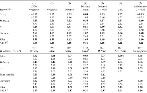
I estimate regression (11) under the five specifications of the spatial matrixW, discussed in Section4.1, and I report the em-pirical results in regressions 1 to 7 in Table1. Regression 1 is estimated with the biased LSDV [see expression (2)] and re-gression 7 is estimated using the Anderson and Hsiao (1982) estimator [see expression (5)]. Regressions 2 to 6 are estimated with the bias-corrected estimatorϕc in expression (4). To im-plementϕc, I estimate the bias correction terms using parame-ter estimates provided by the Anderson and Hsiao (1982) es-timator. Also, the instrument inϕc for the interest ratert, the only endogenous control variable in regressions 1 to 7, is its time-lagged value rt−1. I instrument rt withrt−1 because in unreported results (available upon request) I find that it has the highest correlation withrtacross all the variables in my dataset. 4.3.2 Biased LSDV. To evaluate the empirical importance of the bias correction, regression 1 is estimated with the bi-ased LSDV from expression (2). In this case, the estimates for ρ1,π1, andλ are−0.02, 0.29, and 0.28 respectively. Regres-sion 2 estimates the same model using the bias-corrected esti-mator, and the estimate forρ1,π1, andλ become 0.07, 0.26, and 0.63, respectively. The differences in the estimated para-meters translate into important differences in terms of the eco-nomic implications of the model. In particular, in regression 1, the curvature parameterγ is insignificant (estimate=2.60, t-statistic=1.28), while in regression 2 it is precisely estimated (estimate=1.05,t-statistic=8.27). Thet-statistic forγ is cal-culated using the delta method.
4.3.3 Habit Formation. The estimation results in regres-sions 2 to 6 in Table1reveal that the parameter of the external-habit measure is statistically significant. In particular, when the habit is based on the consumption of neighboring states (W=Wn), the estimate ofρ1is 0.26 (t-statistic=2.50). This
Table 1. Testing habit formation using U.S. state data for 1966–1998
(1) (2) (3) (4) (5) (6) (7)
LSDV Distance Distance AH distance
Type ofW: Neighbors Neighbors Distance urban U>60% USA U>60%
ct−1 −0.02 0.07 0.05 0.04 0.03 0.07 −0.03
−0.53 1.60 1.16 1.05 0.66 1.52 −0.75
W ct−1 0.29 0.26 0.33 0.34 0.37 0.34 0.60
3.70 2.50 2.61 2.73 3.14 2.12 2.64
rt 0.28 0.63 0.61 0.61 0.59 0.62 0.91
1.82 3.89 3.81 3.77 3.68 3.87 1.50
Curvature 2.60 1.05 1.02 1.02 1.02 0.96 0.48
1.28 8.27 7.57 7.45 7.31 6.33 2.00
RRA 3.55 1.59 1.63 1.65 1.69 1.63 1.10
Adj.R2 0.06 0.16 0.16 0.16 0.16 0.15 0.15
(8) (9) (10) (11) (12) (13) (14)
W=Dist.,U>60% US serv inct inct−1 ( ct)2 W inct c− inc No neighbors
ct−1 0.02 0.05 0.04 0.03 0.04 0.001 0.05
0.57 1.15 0.91 0.65 1.01 0.01 1.05
W ct−1 0.40 0.42 0.40 0.31 0.39 0.34 0.36
2.58 2.11 3.02 2.17 2.06 3.19 2.86
rt 0.63 0.66 0.60 0.57 0.62 0.20 0.59
2.76 2.00 3.62 3.39 1.92 1.55 3.66
Extra variable −0.20 −0.19 −0.05 4.08 −0.12
−0.26 −0.28 −0.50 0.56 −0.18
Curvature 0.92 0.79 0.93 1.16 0.91 3.39 1.00
3.43 1.82 5.99 7.23 1.67 0.52 7.05
RRA 1.59 1.51 1.68 1.77 1.61 5.12 1.68
Adj.R2 0.17 0.19 0.17 0.31 0.17 0.04 0.16
NOTE: The table presents parameter estimates (bold face font) and theirt-statistics (below the estimates). Regression 1 uses the LSDV. Regression 7 is estimated with the AH estimator. Regressions 2 to 6 and 8 to 14 are estimated with theϕcestimator. In regressions 1 to 7 and 13 to 14,rtis the control variable, and its instrument inϕcisrt−1. Regressions 8 to 12
include additional control variables. Regression 13 is the same as 5 with cbeing replaced by c− inc. The table reports the within-variation adjusted R-squared, the curvature parameterγ(standard error calculated with delta method), and the RRA coefficient.
estimate increases to 0.33 (t-statistic=2.61) for the distance-weightedW and to 0.34 (t-statistic=2.73) when the degree of urbanization is incorporated in the distance-weighted spa-tial matrix (W=Wd,u). The estimated ρ1 slightly increases when states with a low degree of urbanization are deleted from the distance-weighted and urban-weighted spatial matrix (estimate=0.37,t-statistic=3.14). However, the estimate of ρ1decreases to 0.34 (t-statistic=2.12) when the habit is mea-sured by the average consumption of all states but the state in question (W=Wusa).
The previous results show that the closer two states are, the more they influence one another. Moreover, they suggest that the more urban a state is, the more it seems to influences the other states. The finding that geographical proximity affects the external consumption habit is consistent with existing work (Case1991; Ravina2007). The suggestive evidence that urban centers might drive habits is a new result.
Moving to the internal habit, the estimation shows that in the presence of external-habit formation, the internal habit is sta-tistically insignificant—across regressions 2 to 6 the parameter estimate on the time-lagged dependent variable does not ex-ceed 0.07, and itst-statistic does not exceed 1.60. This find-ing is consistent with existfind-ing empirical studies that estimate pure internal-habit models withannualdata. For example, Fer-son and Constantinides (1991) use national U.S. data and find only weak evidence of internal-habit formation at the annual
frequency. Dynan (2000) finds no evidence for internal-habit formation in individual annual consumption data.
Studies that estimate habit models with quarterly national data, however, report supporting evidence for internal-habit models. For example, see Ferson and Constantinides (1991), Ferson and Harvey (1992), and Grishchenko (2007). Combin-ing the findCombin-ings with annual and quarterly data, one concludes that the impact of the internal habit must be short-lived because it manifests itself at the quarterly frequency and it disappears at the annual frequency.
One reason for failing to accept the internal-habit formation assumption may be the fact that my measure of internal-habit formation does not include many consumption lags. Therefore, I include an additional time lag of own consumption growth, ct−2, to regression 5. In untabulated results, available on request, the parameter estimates for the internal-habit terms ct−1 and ct−2 are again statistically insignificant. In con-trast, the parameter estimate on the external component of the habit is precisely estimated. See Korniotis (2007) on how to use the bias correction approach to estimate a dynamic panel model with fixed effects and higher order lagged-dependent variables and spatially lagged-dependent variables.
4.3.4 Elasticity of Intertemporal Substitution. The coeffi-cient on the log real interest rate provides an estimate for the elasticity of intertemporal substitution (EIS). The estimate of the EIS is significantly different from zero at the 5% confidence
level in regressions 2 to 6. Its value is positive and around 0.61. This estimate is higher than the estimates found using U.S. na-tional data (Hall1988) and is in line with estimates from studies using individual data (e.g., Zeldes1989; Attanasio and Weber 1995; and Vissing-Jorgensen2002).
The estimates on the habit measures and the EIS provide an estimate for the curvature parameterγ because the EIS equals (1−π1−ρ1)/γ. Using the last expression, the implied estimate of γ is around 1.01 across regressions 2 to 6. The estimated γ is also statistically significant at the 5% level (the standard error forγ is calculated using the delta method). The estimate ofγ implies that the coefficient of relative risk aversion, which is given byγ /Sit,Sit=1−(ρ1WiCt−1+π1Ci,t−1)/Cit, is on average 1.60 across regressions 2 to 6. This value is reasonable and within the range used in the literature. For example, see Campbell and Cochrane (1999).
4.3.5 Instrumental Variables. An alternative to the bias-correction estimation is the instrumental variables approach, which produces similar results to the bias-corrected estimator. Following Anderson and Hsiao (1982), I factor out the fixed ef-fects by taking first differences of the linearized Euler equation in (11): 2ct=ρ1[W 2ct−1] +π1[ 2ct−1] + λ1 rt+ ηt, where 2 denotes second-order differences ( 2xτ = xτ −
2xτ−1+xτ−2). Also, the instruments for W 2ct−1, 2ct−1, and rt, are W ct−2, ct−2, and rt−2, respectively. The Anderson and Hsiao (1982) estimates are reported in regres-sion 7. As in regresregres-sion 5, ρ1 is significant (estimate=0.60, t-statistic=2.64) and π1 is insignificant (estimate= −0.03, t-statistic= −0.75). Also, the estimate of the EIS (=0.91, t-statistic=1.50) implies a statistically significant estimate for γ (=0.48,t-statistic=2.00).
Because both the Anderson and Hsiao (1982) and bias-corrected estimators are consistent, the similarities in their qual-itative results are not surprising. However, the bias-corrected estimator provides more precise estimates for the ρ1, γ, and EIS. This finding is confirmed by the simulation results in Sec-tion 5, in which the standard deviation of the Anderson and Hsiao (1982) estimates are found to be higher than the standard deviation of the bias-corrected estimates.
4.4 Robustness Analysis
Overall, the evidence for internal-habit formation is weak. However, the evidence for external-habit formation based on geographical proximity and degree of urbanization is more sub-stantial. I test the robustness of these conclusions by focusing on the distance-weighted and urban-weightedWthat excludes states with a low degree of urbanization, that is, W=Wd,60 (Table1, regressions 8–14).
These regressions are estimated with the bias corrected LSDV. To implementϕc, I estimate the bias correction terms using parameter estimates provided by the Anderson and Hsiao (1982) estimator. All regressions include the interest rates as a control variable and inϕcthe instrument for the interest ratert is its time-lagged valuert−1.
Besidesrt, regressions 8 to 12 include an additional control variable. In particular, regression 8 includes the growth rates of U.S. services. Its instrument inϕc is the average growth rate of the past state income Wd,60 inct−1 ( inct−1 is a vector
with the growth rates of lagged state income across all states). Regression 9 includes the growth rate of state income, inct, and its instrument inϕcisWd,60 inct−1. Regression 10 adds the growth rate of time-lagged state income, inct−1, which is instrumented inϕcby inct−1. Regression 11 includes the squared consumption growth rate and its instrument inϕcis the average squared time-lagged consumption growth rate across all states but the state in question. Regression 12 includes the average income growth rate of the states that determine the habit,Wd,60 inct. Its instrument inϕcisWd,60 inct−1. I use the aforementioned instruments because in unreported results (available upon request), I find that they are highly correlated with the variables they are instrumenting.
4.4.1 Services. State consumption growth is measured with error because it is equal to the growth rate of state re-tail sales, which excludes the growth rate of services. Thus, the growth rate of services at the state level is an omitted vari-able. To account for this omission, regression 8 includes the growth rate of U.S. services. Because the growth rate of U.S. services should be correlated to the consumption of services at the state level, it can alleviate potential omitted variable bi-ases. Conditional on the growth rate of U.S. services, I find that the external-habit term remains significant (estimate= 0.40,t-statistic=2.58), the internal-habit term is insignificant (estimate=0.02,t-statistic=0.57), and the EIS is significant (estimate=0.92,t-statistic=3.43). The issue of measurement error is further investigated in the simulation analysis in Section 5.2.
4.4.2 Income Expectations. The literature finds that con-sumption growth is excessively sensitive to income growth, that is, current consumption growth is related to current in-come growth (e.g., Flavin 1981). One reason for this phe-nomenon is that current income growth can help predict fu-ture income growth, which influences current consumption growth. It is therefore possible that the external-habit mea-sure is significant because it captures some common dimen-sion of economic activity that helps agents forecast their fu-ture income. To control for the excess sensitivity of consump-tion growth to income growth, regression 9 includes state in-come growth as an additional regressor. This estimation shows that the external component of the habit remains significant in the presence of state income growth (ρ1 estimate =0.42, ρ1 t-statistic=2.11).
4.4.3 Liquidity Constraints. The economic model in Sec-tion 4.1 ignores liquidity constraints. If liquidity constraints bind simultaneously across all U.S. states, because of a nega-tive national income shock, consumption growth rates across all states will decrease. If the negative income shock is long-lived (persistent), state consumption levels might remain low for more than one period. In this case, the low consumption growth rate of a state will be correlated with the low past con-sumption growth rates of other state in the absence of external-habit formation. I find that this is not the case in my estima-tion. In line with Zeldes (1989) and Deaton (1991,1992), I ac-count for liquidity constraints by adding the growth rate of time-lagged state income in regression 10. In this regression, ρ1 is 0.40 and it remains statistically significant (t-statistic= 3.02).
4.4.4 Precautionary Savings. Carroll (1997) argues that individuals save due to precautionary motives to finance con-sumption in unforeseen bad states of the economy. Follow-ing Dynan (1993), I measure consumption uncertainty by the squared consumption growth rate, which I add to the estima-tion in regression 11. Like Dynan (1993) and Ravina (2007), I find that the squared consumption growth rate is insignificant. In addition, as in regression 5, the coefficient on the external habit remains significant (estimate=0.31,t-statistic=2.17). These findings rule out the possibility that the external-habit measure is significant because it captures some dimension of overall consumption uncertainty.
4.4.5 Common Shocks. Next, I consider the effect of un-observed common shocks on the significance of the external-habit measures. When common shocks are independent across time, they create cross-sectional correlations in the error term. When they are autocorrelated, they also create autocorrelation in the error term. In both cases, the error term is not iid and Condition1(1) is violated.
Since the corrected estimator does not account for the pres-ence of common shocks directly, I modify regression (11) in one of two ways to factor out the impact of common shocks. First, I use control variables that should be correlated with the common shocks. Second, I estimate regression (11) with modi-fied (relative) state consumption data that are less influenced by common shocks compared to actual state consumption data.
I use state-level income growth rates to purge the effects of common shocks from the error term because income growth determines consumption growth, and thus unobserved income shocks are the source of unobserved consumption shocks. In particular, regression 12 adds Wd,60 inct to the estima-tion. The variableWd,60 inct is the average income growth rate of the states that are included in the definition of the external-habit measure. Thus, it can capture common income shocks that might otherwise have been captured by the exter-nal habit measure. In regression 12, the coefficient estimate on the external-habit measure is 0.39, and its statistical sig-nificance (t-statistic=2.06) is not affected by the presence of Wd,60 inct.
A different way to factor out common shocks is to esti-mate the baseline regression in (11) by replacing consumption growth with relative consumption growth cR(regression 13). Similar to Ostergaard, Sorensen, and Yosha (2002), relative consumption growth, cR, is the difference between state con-sumption growth and state income growth. Because income growth includes any common unobserved shocks that matter for consumption growth, the variation in relative consumption growth is primarily state specific. In this case, the estimation shows that the relative habit growthWd,60 cR,t−1 is statisti-cally significant in explaining relative consumption growth cR (ρ1estimate=0.34,ρ1t-statistic=3.19).
4.4.6 Cross-Border Shopping. In a final robustness test, I find that potential cross-border shopping has no impact on the significance of the external component of the habit. Cross-border shopping can cause spending in two neighboring states to be positively correlated, independent of any external-habit effects. For example, a positive income shock in Connecticut increases the purchasing power, and subsequent consumption, of Connecticut residents. It is reasonable to assume that some of
this excess purchasing power will be spent in neighboring states such as New York. To factor out the effect of cross-border shop-ping, I exclude the neighboring states from the distance-based, urban-based, external-habit measure that omits states with low degree of urbanization. In regression 14, the parameter esti-mate on the external-habit term is again precisely estiesti-mated (estimate=0.36,t-statistic=2.86).
5. FINITE–SAMPLE PERFORMANCE
Having estimated the regression with habit formation, I con-duct a simulation exercise based on the empirical results in Sec-tion4. The simulations analyze the finite-sample properties of the bias-corrected estimatorϕcwith and without measurement error in the dependent variable.
5.1 Simulation Set-Up
In the case of no measurement error, the data-generating mechanisms (DGM) of theN×1 vector of dependent variables Yt and theN×1 vector of endogenous control variables Xt are
Yt=π1Yt−1+ρ1(WYt−1)+λXt+c+ηt and (12a)
Xt=α1Xt−1+α0 +ηx,t. (12b) Here,ηtis given by ζ (εcom,t+εt), andηx,t is given byεx,t+
αηxεcom,t. The error terms εx,t,εcom,t, andεt are all iid nor-mally distributed with a mean of zero and a variance of 1. Also, π1=0.03,ρ1=0.37,λ=0.59,ci∼NIID(0.01,1),α1=0.78, α0i∼NIID(0.014,1),αηx=0.33, andζ =2.01. The values of π1,ρ1, andλare from Table1, regression 5. TheN×1 vector
ccontains the fixed effectsci, which are drawn from a normal distirbution. The mean of the normal distribution is the cross-sectional average of the mean consumption growth rate across the U.S. states. TheN×NmatrixWis given byWd,60.
As in regression 5 in Table 1, the simulation has only one control variableXt, which is defined to reflect the properties of the log real interest rate. The DGM ofXtfollows the pooled dy-namic AR(1) process in (12b). TheN×1 vectorα0is a vector containing the fixed effectsα0i, which are drawn from a normal distribution. Its mean is the cross-sectional average of the mean log real interest rate across the U.S. states. The value forα1is the estimate from an AR(1) pooled dynamic panel model with fixed effects on the log real interest rate. The AR(1) is estimated using the procedure in Hahn and Kuersteiner (2002).
The error terms ηt [=ζ (εcom,t+εt)] and ηx,t (=εx,t +
αηxεcom,t) are correlated because they both include the com-mon shock εcom,t. Also, the parameterζ inηt, and the para-meterαηxinηx,t are chosen to match two facts: (a) the ratio of the variances (RATIO) of the log real interest rate and estimated residualηfrom regression 5 in Table1, and (b) the correlation betweenXtandηt(CORxη). Then, using the expressions forYt,
ηt, andηx,t, αηx=
21−α 2 1 COR2xη −1
−1/2
=0.33 and
ζ =
1+α2
ηx 2(1−α21)RATIO
1/2 =2.01,
because in regression 5, the levels of RATIO andCORxη are
0.35 and 0.28, respectively.
Using the above set-up, four cases are simulated under four values ofT: 20, 30, 40, and 60. In each case, 20,000 draws are executed. Each draw generatesT+100 observations for each cross-sectional unit. The first 100 observations are deleted to mitigate the effects of the initial conditions. For every draw, the sample ofTobservations is used to estimateπ1,ρ1, andλ.
Three estimators are considered. The first estimator is the biased LSDV from expression (2). The second is the bias-correctedϕc, which is implemented in the way described in Section 3.3. The third is the Anderson and Hsiao (1982) in-strumental variables estimator ϕAH from expressions (5). In
ϕAH, the instruments for Yt−1,W Yt−1, and Xt, areYt−2,
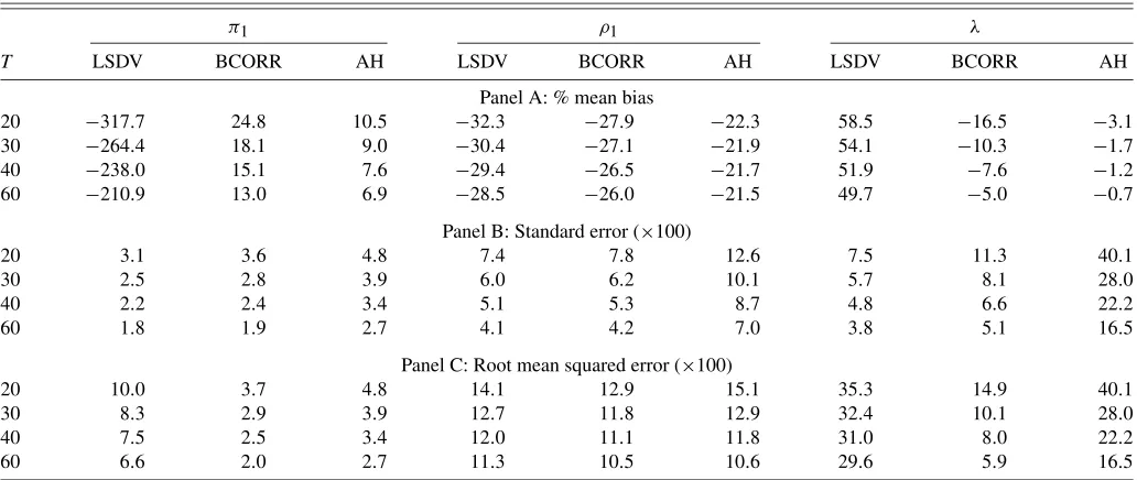
WYt−2, andXt−2 respectively. For each of the three estima-tors, the percentage mean bias, standard error, and root mean squared error (RMSE) ofπ1,ρ1, andλare calculated with their estimates from the 20,000 draws (Table 2, with no measure-ment error; Table3, with measurement error). In what follows, I denote the Anderson and Hsiao (1982) estimator by AH.
5.2 Results With No Measurement Error
When the dependent variable is accurately measured, the LSDV is severely biased, but it has a low standard error and RMSE. The bias-correctedϕchas a low finite-sample bias, to-gether with a low standard error and RMSE. The AH estimator has the smallest bias. Because it has the highest standard error however, its RMSE is higher than the RMSE ofϕc.
The previous findings are drawn from the simulation results reported in Table2. Consider the case withT=30. Forρ1, the percentage bias is the highest for LSDV (−30.4), and it is the smallest for the AH (−21.9). It is also only−27.1 for the bias-corrected estimator. However, in terms of the variability ofρ1, the LSDV has the smallest standard error (6.0), and the AH has
the highest standard error (10.1). The standard deviation for the bias-corrected estimator is only 6.2, and it is very close to that of the LSDV. Finally, for ρ1, theϕc has the smallest RMSE (11.8) and the AH has the highest RMSE (12.9). Similar results hold forπ1andλ.
The findings of the simulation exercise reveal that the bias-corrected estimator retains the low variance of the unbias-corrected LSDV, while it has a significantly lower bias. The low variance of the LSDV is the motivation for Kiviet (1995) to pursue the bias correction approach in the context of dynamic panel mod-els with no spatially lagged dependent variables and no endoge-nous control variables.
5.3 Results With Measurement Error
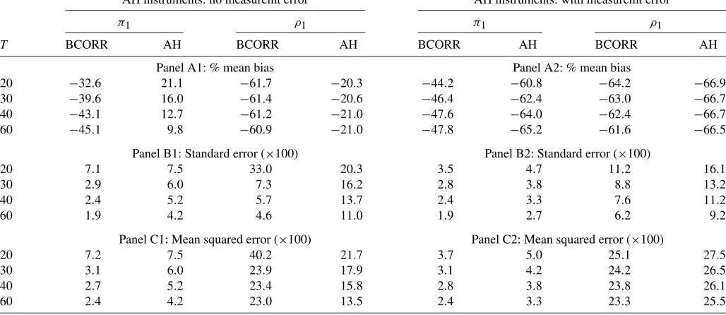
A set of simulation results quantify the effect of measurement error on the finite-sample performance of the bias-corrected es-timator and the AH eses-timator. In these simulations, the observed value ofY,Yobs, isYobs=Y∗+v,v∼NIID(0,σv2). The vari-ableY∗ is the true value ofYand v is the measurement er-ror. The variance ofvisσv2, and its level is chosen so that the signal-to-noise ratio is 1 for all cross-sectional units. Also, the measurement error is orthogonal to error termsη[from Equa-tion (12a)] andηx[from Equation (12b)]. To focus on the effect of measurement error inY, I assume thatXis free of measure-ment error (Xobs=X∗). The values forY∗andX∗are generated as in the case of no measurement error presented in Section5.1. The simulation results for theϕc and the AH estimators are of two types (Table3). In the type 1 simulations, the instruments for the AH do not suffer from measurement error, that is, the instruments for Yobs,t−1,W Yobs,t−1, and Xobs,t, areY∗t−2,
WY∗t−2, andX∗t−2, respectively. In practice, of course, it might be almost impossible to find such instruments. Nevertheless, the type 1 simulations can illustrate whether the corrected LSDV can perform better than the AH, which uses the best possible
Table 2. Simulation results: no measurement error
π1 ρ1 λ
T LSDV BCORR AH LSDV BCORR AH LSDV BCORR AH
Panel A: % mean bias
20 −317.7 24.8 10.5 −32.3 −27.9 −22.3 58.5 −16.5 −3.1 30 −264.4 18.1 9.0 −30.4 −27.1 −21.9 54.1 −10.3 −1.7 40 −238.0 15.1 7.6 −29.4 −26.5 −21.7 51.9 −7.6 −1.2 60 −210.9 13.0 6.9 −28.5 −26.0 −21.5 49.7 −5.0 −0.7
Panel B: Standard error (×100)
20 3.1 3.6 4.8 7.4 7.8 12.6 7.5 11.3 40.1
30 2.5 2.8 3.9 6.0 6.2 10.1 5.7 8.1 28.0
40 2.2 2.4 3.4 5.1 5.3 8.7 4.8 6.6 22.2
60 1.8 1.9 2.7 4.1 4.2 7.0 3.8 5.1 16.5
Panel C: Root mean squared error (×100)
20 10.0 3.7 4.8 14.1 12.9 15.1 35.3 14.9 40.1
30 8.3 2.9 3.9 12.7 11.8 12.9 32.4 10.1 28.0
40 7.5 2.5 3.4 12.0 11.1 11.8 31.0 8.0 22.2
60 6.6 2.0 2.7 11.3 10.5 10.6 29.6 5.9 16.5
NOTE: The table presents simulation results forT= {20,30,40,60}. Three estimators are considered, the LSDV, the bias-correctedϕc(BCORR), and the estimator by Anderson– Hsiao (1982) (AH). The table reports the percentage mean bias, which is the average of[(ϕ−ϕ)/ϕ] ×100,ϕandϕdenote the true and estimated values ofπ1,ρ1, andλ(panel A). I also calculate the standard error ofϕ(panel B), and their root mean squared error, which is the square root of the average of(ϕ−ϕ)2(panel C). The values of the standard errors and root mean squared errors in panels B and C are multiplied by a 100.
Table 3. Simulation results: with measurement error
Type 1 Type 2
AH instruments: no measuremt error AH instruments: with measuremt error
π1 ρ1 π1 ρ1
T BCORR AH BCORR AH BCORR AH BCORR AH
Panel A1: % mean bias Panel A2: % mean bias
20 −32.6 21.1 −61.7 −20.3 −44.2 −60.8 −64.2 −66.9 30 −39.6 16.0 −61.4 −20.6 −46.4 −62.4 −63.0 −66.7 40 −43.1 12.7 −61.2 −21.0 −47.6 −64.0 −62.4 −66.7 60 −45.1 9.8 −60.9 −21.0 −47.8 −65.2 −61.6 −66.5
Panel B1: Standard error (×100) Panel B2: Standard error (×100)
20 7.1 7.5 33.0 20.3 3.5 4.7 11.2 16.1
30 2.9 6.0 7.3 16.2 2.8 3.8 8.8 13.2
40 2.4 5.2 5.7 13.7 2.4 3.3 7.6 11.2
60 1.9 4.2 4.6 11.0 1.9 2.7 6.2 9.2
Panel C1: Mean squared error (×100) Panel C2: Mean squared error (×100)
20 7.2 7.5 40.2 21.7 3.7 5.0 25.1 27.5
30 3.1 6.0 23.9 17.9 3.1 4.2 24.2 26.5
40 2.7 5.2 23.4 15.8 2.8 3.8 23.8 26.1
60 2.4 4.2 23.0 13.5 2.4 3.3 23.3 25.5
NOTE: The table presents simulation results for estimatingYobs,t=π1Yobs,t−1+ρ1WYobs,t−1+λX∗t+c+ηt. TheYobs,t=Y∗t +vt, whereYobs,tis the observed value of the dependent variable,Y∗t is its true, andvtis the measurement error. I consider the bias-corrected correctedϕc(BCORR), and the estimator by AH (1982). In type 1, the instruments for the AH areY∗t
−2,WY∗t−2, andX∗t−2. In type 2, the instruments for the AH areYobs,t−2,WYobs,t−2, andX∗t−2. The table reports the mean bias (panels A1 and A2), standard deviation
(panels B1 and B2), and root mean squared error (panels C1 and C2) in the same way as in Table2. The standard errors and root mean squared errors are multiplied by a 100.
instruments, that is, instrument with no measurement error. In the type 2 simulations, the instruments for the AH are subject to measurement error, that is, the instruments for Yobs,t−1,
W Yobs,t−1, and Xobs,t, areYobs,t−2,WYobs,t−2, andX∗t−2, respectively. Because the bias vector inϕc is computed using the AH, the value ofϕc is different between the type 1 and type 2 simulations. The simulation results forλare similar to those reported in Table2, and are omitted from Table3.
Forπ1, in the type 1 simulations, theϕcis more biased than AH. The result is not surprising because in the presence of mea-surement error theϕc is inconsistent, while the AH is consis-tent. However, the bias-corrected estimator has a smaller stan-dard deviation and RMSE than the AH that uses instruments, which are free of measurement error. Moving to the type 2 sim-ulations, the AH estimate ofπ1has a high percentage bias be-cause the instruments for AH are subject to measurement error. Also, the standard error and RMSE of the AH are higher than those of the bias-corrected estimator.
Forρ1, in the type 1 simulations, the percentage finite-sample bias for the bias-corrected estimator is higher than the AH, and its standard deviation is lower than the AH. However, its RMSE is slightly higher than the AH. Moving to the type 2 simulations, the bias-corrected estimator now has a smaller percentage bias, standard deviation, and RMSE than the AH.
Overall, the results show that in the presence of measurement error, the bias-corrected estimator maintains fairly good finite-sample properties. Also, compared to the AH, it always has a smaller standard error.
6. CONCLUSION
A leading explanation of aggregate stock market behavior states that asset returns are determined as if consumers’ wel-fare depends on the difference between actual consumption and
a habit level of consumption. In some models, the habit is de-termined by the consumer’s past consumption (internal-habit formation). In other models, it is determined by the consump-tion of others (external-habit formaconsump-tion). To test for the relative strength of these two types of habit formation, this paper pro-poses an estimator for dynamic panel models with fixed effects, spatial effects, and endogenous regressors.
The estimator is based on the bias-correction method of Hahn and Kuersteiner (2002) for dynamic panel models with only fixed effects. I modify their approach to accommodate spatial effects and endogenous control variables. The proposed bias-corrected estimator is a hybrid of the least-squares dummy vari-able estimator of Hahn and Kuersteiner (2002) and the instru-mental variables estimator of Anderson and Hsiao (1982). Like Hahn and Kuersteiner (2002), I use de-meaned data to elimi-nate the fixed effects, and like Anderson and Hsiao (1982), I in-strument the endogenous control variables. I show that the new estimator is consistent, has no asymptotic bias, and is asymptot-ically normally distributed. It also has good finite sample prop-erties.
I apply the estimator to consumption data for the 48 continen-tal U.S. states to test for habit formation at the aggregate level. The estimation considers both internally and externally deter-mined habits. The internal-habit level of a state is measured by its own time-lagged consumption growth. The external-habit level of a state is measured by various weighted averages of time-lagged consumption growth rates of other states. The es-timation finds weak evidence for internal-habit formation and strong evidence of external-habit formation. In particular, the farther apart two states are, the less they influence one another. Furthermore, states with population that predominantly lives in urban centers seem to affect the consumption of other states the most. The suggestive evidence that consumption trends might