Full Terms & Conditions of access and use can be found at
http://www.tandfonline.com/action/journalInformation?journalCode=ubes20
Download by: [Universitas Maritim Raja Ali Haji] Date: 11 January 2016, At: 19:25
Journal of Business & Economic Statistics
ISSN: 0735-0015 (Print) 1537-2707 (Online) Journal homepage: http://www.tandfonline.com/loi/ubes20
Semiparametric Conditional Quantile Estimation
Through Copula-Based Multivariate Models
Hohsuk Noh, Anouar El Ghouch & Ingrid Van Keilegom
To cite this article: Hohsuk Noh, Anouar El Ghouch & Ingrid Van Keilegom (2015)
Semiparametric Conditional Quantile Estimation Through Copula-Based Multivariate Models, Journal of Business & Economic Statistics, 33:2, 167-178, DOI: 10.1080/07350015.2014.926171
To link to this article: http://dx.doi.org/10.1080/07350015.2014.926171
Accepted author version posted online: 12 Jun 2014.
Submit your article to this journal
Article views: 399
View related articles
Semiparametric Conditional Quantile Estimation
Through Copula-Based Multivariate Models
Hohsuk N
OH, Anouar E
LG
HOUCH, and Ingrid V
ANK
EILEGOMInstitut de Statistiqu ´e, Biostatistique et Sciences Actuarielles, Universite catholique de Louvain, Louvain-la-Neuve 1348, Belgium ([email protected]; [email protected]; [email protected])
We consider a new approach in quantile regression modeling based on the copula function that defines the dependence structure between the variables of interest. The key idea of this approach is to rewrite the characterization of a regression quantile in terms of a copula and marginal distributions. After the copula and the marginal distributions are estimated, the new estimator is obtained as the weighted quantile of the response variable in the model. The proposed conditional estimator has three main advantages: it applies to both iid and time series data, it is automatically monotonic across quantiles, and, unlike other copula-based methods, it can be directly applied to the multiple covariates case without introducing any extra complications. We show the asymptotic properties of our estimator when the copula is estimated by maximizing the pseudo-log-likelihood and the margins are estimated nonparametrically including the case where the copula family is misspecified. We also present the finite sample performance of the estimator and illustrate the usefulness of our proposal by an application to the historical volatilities of Google and Yahoo.
KEY WORDS: Check function; Dependence modeling; Markov process; Pseudo-log-likelihood; Vine copulas.
1. INTRODUCTION
Appropriate understanding and modeling of the dependence structure between financial assets is an important task. Espe-cially, the characterization of the conditional dependence be-tween random variables at a given quantile constitutes an im-portant ingredient in modern risk management. As a copula has emerged as an effective tool to model dependence between nonelliptic and ftailed random variables, several authors at-tempted to propose conditional quantile estimation methods which are able to make use of the advantages of copulas in de-pendence modeling. Their common starting point is that since the copula function holds all information on the different forms of dependence between random variables, the form of the con-ditional quantile relationship is implied by the copula joining those random variables.
Some examples of such work include Bouy´e and Salmon (2009), Chen and Fan (2006), and Chen, Koenker, and Xiao (2009). In an earlier version of Bouy´e and Salmon (2009), the authors explicitly showed the link between the form of the con-ditional quantile relationship and the copula function for sev-eral well-known copula families such as elliptical copulas and Archimedean copulas. Further, they illustrated how such link can be used in conditional quantile estimation both when mod-eling the interdependence between random variables and when modeling the temporal dependence between them. Focusing more on the latter case, Chen and Fan (2006) studied a class of univariate copula-based stationary Markov models. Under the assumption of correct specification of the parametric copula, Chen and Fan (2006) established asymptotic properties of their quantile regression estimator when the copula is estimated by maximizing the pseudo-log-likelihood and the marginals are es-timated nonparametrically. Additionally, also in the time series context, Chen, Koenker, and Xiao (2009) employed parametric copula models to propose several distinct nonlinear quantile
au-toregression models and investigated the asymptotic properties of their estimator when both the copulas and the marginals could be globally misspecified but assuming the correct specification of a conditional quantile function at a particular quantile.
However, all these works consider a conditional quantile given just one covariate such as the conditional quantile of Y givenX or the conditional quantile of Yt given its lagged observationYt−1. Nevertheless, often it is necessary to consider
multivariate quantile regression conditioning on more than one covariate. Apart from examples in the iid setup, there are many such examples in the time series setting where the copula-based quantile estimation methods should be extended. One example is a copula-based Markov process of higher order, for which Ibragimov (2009) studied how a copula characterizes the statis-tical properties of the corresponding Markov process. However, they did not investigate the issue of the conditional quantile estimation there. Another example is copula-based multivari-ate time series models, where for instance the dependence between two Markovian (stationary) time series Xt and Yt is modeled via a copula which characterizes the dependence be-tweenXt−1, Yt−1, Xt, andYt, in other words, serial dependence and interdependence between two time series. R´emillard, Pa-pageogiou, and Soustra (2012) discussed parameter estimation and goodness-of-fit testing for this model but did not address the issue of quantile estimation such as the conditional quantile ofYtgivenXt−1, Yt−1, andXt.
Based on this observation, we are motivated to develop an extended version of the previous copula-based quantile regres-sion methods to handle multiple covariates. The key idea of the previous methods is to express the conditional distribution
© 2015American Statistical Association Journal of Business & Economic Statistics April 2015, Vol. 33, No. 2 DOI:10.1080/07350015.2014.926171
167
function in terms of a certain partial derivative of the copula function and the marginal distributions, and obtain the condi-tional quantile through it. Although it is possible to consider an extension based on this idea, we find it better for convenient computation and concise theoretical development to estimate the conditional quantile function directly using the so-called “check” function in Koenker and Bassett (1978) without go-ing through the conditional distribution. The main idea of our new approach is to rewrite the check-function based character-ization of a regression quantile in terms of a copula function and marginal distributions. Actually, our proposal is an exten-sion of the recent work of Noh, El Ghouch, and Bouezmarni (2013) from mean regression to quantile regression. However, nondifferentiability of the check loss function in quantile re-gression makes the extension nontrivial, which needs a separate treatment. Additionally, to broaden the area of application, we derive the asymptotic properties of the estimator under general conditions where both the iid setting and the time series setting can be considered.
The rest of this article is organized as follows. In Section 2, we introduce our conditional quantile estimation method. We present the asymptotic properties of the proposed estimator in Section3 and present the finite sample performance of our estimator via some numerical simulations both in the iid and time series setting in Section4. Finally, we analyze the daily log returns data of Google and Yahoo companies in Section5 to illustrate the usefulness of our proposal. All technical details are deferred to the Appendix.
2. COPULA-BASED QUANTILE REGRESSION ESTIMATOR
Let X =(X1, . . . , Xd) be a covariate vector of dimension
d ≥1 andYbe a response variable with continuous cumulative distribution functions (cdf) F1, . . . , Fd, and F0, respectively.
We denote the density ofXj andY byfj andf0, respectively. For a givenx =(x1, . . . , xd)⊤, from the seminal work of Sklar
(1959), the cdf of (Y,X) evaluated at (y,x) can be expressed as
C(F0(y),F(x)).Here,F(x)=(F1(x1), . . . , Fd(xd))⊤andCis
the copula distribution of (Y,X) defined byC(u0, u1, . . . , ud)=
P(U0 ≤u0, U1≤u1, . . . , Ud ≤ud), where U0=F0(Y) and
Uj =Fj(Xj), j=1, . . . , d. The copulaCis considered to hold all information on the dependence of (Y,X) since it joins the
marginals together to give the joint distribution. Naturally, it is expected that a given copula function implies a certain form of the conditional quantile relationship.
More precisely, the following link holds between the copula and the conditional distribution when the dimension ofXis one:
∂C(u0, u1)
∂u1 =FY|X1
F0−1(u0)F1−1(u1),
whereFY|X1is the conditional distribution ofYgivenX1. From
this link, the conditional quantile function mτ(x1) ofY given
X1=x1 is derived in terms of the copula function and the marginals:
mτ(x1)=F0−1(QU0|U1(τ|F1(x1))), (1)
whereQU0|U1(τ|u1) is the conditionalτ-quantile function ofU0
givenU1=u1, which is the inverse function of∂C(u0, u1)/∂u1
with respect tou0. The expression (1) is the key idea underlying the previous works (Chen and Fan2006; Bouy´e and Salmon 2009; Chen et al.2009). Although it is possible to consider the extension of the relation (1) to multiple covariate case (d ≥2), we use another link between the conditional quantile and the copula via the check function to propose an extension which has computational convenience and for which concise asymptotic theory can be easily developed.
For that purpose, we note that from the definition of copula function, the conditional density ofYgivenX=xis expressed
as
f0(y)
c(F0(y),F(x))
cX(F(x))
, (2)
where c(u0,u)≡c(u0, u1, . . . , ud)=∂d+1C(u0, u1, . . . , u
d)/
∂u0∂u1. . . ∂ud is the copula density corresponding to C and
cX(u)≡cX(u1, . . . , ud)=∂dC(1, u1, . . . , ud)/∂u1. . . ∂ud is the copula density of X. Interestingly, thanks to the
expres-sion (2), theτ-conditional quantilemτ(x) ofYgivenX =xcan be written in terms of the copula and the marginals as follows:
mτ(x)=arg min a
E[ρτ(Y −a)|X =x]
=arg min a
E[ρτ(Y −a)c(F0(Y),F(x))], (3)
whereρτ(y)=y(τ−I(y <0)) is the well known check func-tion. Note that different from (1), the expression (3) is not af-fected by the dimension of the covariate vectorX.
If ˆc, ˆF0, and ˆFj are any given estimators forc,F0, andFj,
j =1, . . . , d, respectively, thenmτ(·) can be estimated by
ˆ
mτ(x)=arg min a
n
i=1
ρτ(Yi−a) ˆc( ˆF0(Yi),Fˆ(x)), (4)
where ˆF(x)=( ˆF1(x1), . . . ,Fˆd(xd))⊤. Note that the estimator in
(4) has the monotonicity across quantile levels. It can be shown using the argument in the proof of Theorem 2.5 of Koenker (2005). Following the argument there, one can prove that
(τ2−τ1)( ˆmτ2(x)−mˆτ1(x))
n
i=1
ˆ
c( ˆF0(Yi),Fˆ(x))≥0.
Since ˆc≥0, this implies that ˆmτ2(x)≥mˆτ1(x) wheneverτ2≥
τ1.
Since there are many different methods available in the lit-erature for estimating a copula and a cdf, ˆm(x) can be a
non-parametric or a seminon-parametric or a fully non-parametric estimator depending on the method of estimating the components in (4). In this article, we consider a semiparametric approach where the copula is parameterized but the marginal distributions are left unspecified as in Noh, El Ghouch, and Bouezmarni (2013). Specifically, we assume a certain parametric family of copula densities,C= {c(u0,u;θ), θ∈}, whereis a compact
sub-set ofRp, to which the true copula density belongs or by which it is well approximated.
3. ASYMPTOTIC PROPERTIES OF THE PROPOSED ESTIMATOR
In this section, we first provide general assumptions about the estimator, which will allow us to investigate its asymptotic
properties both in the iid and dependent settings. Then, we will present the asymptotic representation of the estimator derived from the assumptions.
3.1 Assumptions
Before stating the assumptions, we introduce some notations, which will be used throughout the asymptotic analysis of our estimator. As mentioned in the previous section, we consider a certain family of copula densities,C= {c(u0,u;θ), θ∈}, for
estimating the true densityc(u0,u). Defineθ∗to be the (unique)
pseudo-true copula parameter which lies in the interior ofand minimizes
Here, I(θ) is the classical Kullback-Leibler information cri-terion expressed in terms of copula densities instead of the traditional densities. It is clear that when the true copula density belongs to the given family, that is, c(·)=c(·;θ0)
Concerning the partial derivatives of the copula density, we define
Here are the assumptions for our estimator.
(C0) {Yi}i≥1is a strictly stationary process withβ-mixing
Assumption (C3) is satisfied for many popular copula fami-lies. (C4) and (C5) are typically assumed in quantile regression. Hence, in the following we will give some examples where (C0),
(C1), and (C2) are satisfied in the iid setting and the time series setting.
3.1.1 IID Setting. Suppose that we have (Yi,Xi), i= 1, . . . , n, an independent and identically distributed (iid) sam-ple ofnobservations generated from the distribution of (Y,X).
In this case, (C0) is trivially satisfied. Concerning (C1), it is satisfied with the empirical distribution ofXj and its rescaled version which is popular in copula estimation context and is defined by
Additionally, we can also use kernel smoothing method for estimatingFj(·), j =1, . . . , d. Letk(·) be a function which is a symmetric probability density function andh≡hn→0 be a bandwidth parameter. Then, a kernel smoothing estimator ˜Fj is given by
→0 holds for the bandwidth h, then for ˆFj =F˜j, the following condition is satisfied:
(C1’) ˆFj(xj)=n−1ni=1I(Xj,i≤xj)+op(n−1/2), from which (C1) follows. One advantage of using ˜Fj is that it results in a smooth estimate ˆmτ(x), whereas the empirical distribution or its rescaled version does not. As for (C2), one example of the estimator ˆθ that satisfies (C2) in the literature is the maximum pseudo-likelihood (PL) estimator ˆθPL, which
maximizes
was studied by several authors including Genest, Ghoudi, and Rivest (1995), Klaassen and Wellner (1997), Silvapulle, Kim, and Silvapulle (2004), Tsukahara (2005), and Kojadinovic and Yan (2011), etc. If the score function ofc(u0,u;θ) satisfies the
assumptions (A.1)–(A.5) given in Tsukahara (2005), the PL esti-mator satisfies (C2) even when the copula family is misspecified as checked in Noh, El Ghouch, and Bouezmarni (2013).
3.1.2 Time Series Setting. Assumptions under which a copula-based Markov process satisfies α-mixing or β-mixing have been studied by many authors. For example, if {Yi}i≥1
is a (stationary) univariate first-order Markov process and the copula of (Yi, Yi−1)≡(Yi, Xi,1) satisfies certain conditions (see
Proposition 2.1 of Chen and Fan2006), then Assumption (C0) holds and hence (C1) also holds with any estimator ˆFj(·) satis-fying (C1’) (see Rio2000). Following similar ideas, R´emillard, Papageogiou, and Soustra (2012) extended this result to the case of copula-based multivariate first-order Markov process. As for copula-based Markov processes of higher order, unfortunately such results are rare. The only related work that we have found is Ibragimov (2009), who obtained a characterization of higher-order Markov processes in terms of copulas, but he did not discuss the mixing properties of the resulting process.
Concerning Assumption (C2), if we consider an extension of the maximum pseudo-likelihood estimator studied by Genest,
Ghoudi, and Rivest (1995) to the Markovian case, the result-ing estimator satisfies (C2). For example, suppose that we have a sample {(Yi, Xi) :i=1, . . . , n}of a multivariate first-order
then (C2) holds according to Theorem 1 in R´emillard, Papageo-giou, and Soustra (2012) under the assumptions (A1)–(A4) that they provided. For univariate copula-based first-order Markov models, a similar result can be found in Chen and Fan (2006).
3.2 Asymptotic Representation of the Estimator ˆmτ(x)
To realize the theoretical analysis of our estimator, we begin by introducing a few more notations:
• F0ˆ (y)=n−1n
Now we are ready to present the asymptotic representation of the proposed estimator.
Theorem 3.1. Suppose that Assumptions (C0)–(C5) hold. Then, we have
Theorem 3.1 implies that the estimator ˆmτ(x) converges in probability to mτ(x;θ∗) asn→ ∞. Hence, when the copula family is misspecified, the estimator ˆmτ(x) is no more con-sistent. In such situation, since c(·;θ∗) is just the best
ap-proximation to the true copula densityc(·), we have a bias in the estimation of the true conditional quantile functionmτ(x), which is (asymptotically) the difference between mτ(x) and
its best approximation mτ(x;θ∗) among the function class {m(x;θ) :θ∈}.
As an application of Theorem 3.1, we consider the asymptotic normality of the estimator, for which we have to make a stronger assumption than (C2):
(C2′) ˆθ−θ∗=n−1ni=1ηi+op(n−1/2), whereηi =η(U0,i,
Ui;θ∗) is ap-dimensional random vector such thatEη=0and Eη⊤η<∞andUi =(U1,i, . . . , Ud,i)⊤.
This stronger assumption also holds for ˆθPLin the iid setting
and ˆθdepPL in the time series setting with the same conditions for (C2). For the iid case, the functionηis given by
η(U0,U;θ)=J−1(θ)×K(U0,U;θ), (7)
Concerning the time series case, see Chen and Fan (2006) for the univariate case and R´emillard, Papageogiou, and Soustra (2012) for the multivariate case. Replacing (C2) with (C2’) in the previous assumptions, we have an asymptotic linear representation of the conditional quantile estimator ˆmτ(x), which implies the asymptotic normality of ˆmτ(x).
Corollary 3.1. Suppose that Assumptions (C0)–(C1), (C1’), (C2’), (C3)–(C5) hold. Then, we have
√
mτ(x;θ∗)) follows asymptotically a normal distribution with mean 0 and variance σ2
=var(E1)+2j∞=1cov(Ej+1, E1),
where Ei denotes each summand in the summation of (8) (see Rio 2000, theorem 4.2). Especially, since σ2
=var(E1) when the data are iid, we can estimate σ2 by an estimator
ˆ
σ2=n−1ni=1{Ei−n−1
n
i=1Ei}2, where Ei is an estima-tor ofEiobtained by replacing all the unknown quantities inEi by their corresponding estimates, for example,θ∗by ˆθandF0
by ˆF0. Thanks to this estimator ˆσ, we can easily calculate the confidence interval formτ(x;θ∗) using Corollary 3.1.
However, according to our simulation studies (see Section4), the accuracy of the coverage of this confidence interval seems
to sensitively depend on the accuracy of the estimation of the unknown quantities involved inEi. Due to this, we propose to use a bootstrap method to approximate the asymptotic variance of the estimator ˆmτ(x). The bootstrap that we use for the iid data in our simulations is outlined below:
Step 0. Obtain the copula parameter estimate ˆθfrom (5) and the marginal distribution estimates ˜F0 and ˜Fj using the kernel smoothing method with appropriate band-widthsh0,nandhj,n, j =1, . . . , d.
Step 1. Generate n independent random vectors Ubi =
(U0b,i, . . . , Ud,ib )⊤, i=1, . . . , n from the estimated copulac(u0, . . . , ud; ˆθ).
Step 2. Let Yib=F˜0−1(U0b,i) and Xbj,i=F˜j−1(Uj,ib ), j =
1, . . . , d.
Step 3. Repeating Steps 1 and 2 a large number of times, compute the bootstrap values ˆmb
τ(x), b=1, . . . , Bof the estimator ˆmτ(x) and then calculate the estimate of the asymptotic variance using them:
ˆ
Following similar ideas but modifying Steps 0 and 1 (see Section 4.3 in Chen and Fan (2006) and Section2in R´emillard, Papageogiou, and Soustra (2012)), we can estimate the asymp-totic varianceσ2 in the time series setting using a bootstrap procedure. In Section4, we investigate how the proposed boot-strap procedures perform by checking the coverage probabilities of the confidence interval for ˆmτ(x) based on this procedure. In our simulations, we observe that it is important for satisfactory accuracy of the coverage of the confidence interval to use the kernel smoothing estimates of the marginal distributions fol-lowing the concept of the smoothed bootstrap (Silverman and Young1987) in both the iid and time series setting. If we use the empirical distribution or its rescaled version, the coverage prob-ability of the confidence interval does not approach the nominal confidence level at all.
4. NUMERICAL RESULTS
In this section, we first check whether the asymptotic theory for ˆmτ(x) works both in the iid setting and in the time series setting. Second, we compare our semiparametric estimator with some competitors. For this purpose, we consider the following data generating processes (DGP):
• DGP A (F0(Y), F1(X1))∼Clayton copula with paramter α
– The resulting quantile regression function is
mτ(x1)=F0−1
– The resulting quantile regression function is
mτ(x)
Although we describe each DGP with the focus on the iid setting, it can be also described for the time series setting. For example, using DGP A with Y =Yi, X1=Yi−1, and F0=F1=F, we can generate a sample{Yi}ni=1from a
univari-ate first-order Markov model. Then, the conditional quantile function ofYi givenYi−1 =y is given bymτ(y)=F−1((1+
F(y)−α(τ−α/(1+α)−1))−1/α).Table 1shows the parameters of the copula and the marginal distributions of each DGP subspe-cialized from DGPs A and B. All computations are done with R (R Development Core Team2011).
4.1 Verifying the Asymptotic Results about ˆmτ(x)
In this section, to verify the established asymptotic results, we compute a confidence interval formτ(x) either by the asymp-totic representation or the bootstrap proposed in Section3. By verifying whether the empirical coverage probabilities (ECP) of the (1−α)-confidence interval formτ(x) are close to the nom-inal confidence level (1−α), we indirectly check whether the estimator ˆmτ(x) is asymptotically normal.
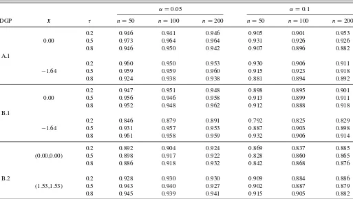
First, concerning the iid setting, we generate 500 random samples of size n=50,100, and n=200 from DGPs A.1, B.1, and B.2 and compute a confidence interval for mτ(x) using ˆσ2 and Corollary 3.1. Table 2 shows the ECP of the
(1−α)-confidence interval formτ(x) withα=0.05 and 0.1. We observe that depending on the location of the covariates and the quantile level, sometimes the ECP has a quite different value from its nominal confidence level. As mentioned before, the main reason for this is the inaccuracy of the estimation of the unknown quantities involved in the asymptotic representation. As is typical in quantile regression, the asymptotic representa-tion for ˆmτ(x) involves the conditional densityfY|X(mτ(x)|x), which is equal tof0(mτ(x;θ∗))c(F0(mτ(x;θ∗)),F(x);θ∗) when the copula family is correct. Since it controls the scale of the es-timated asymptotic variance of ˆmτ(x), the estimation accuracy of it seems to affect the ECP a lot. To confirm our claim, we evaluate the asymptotic representation using the true values of all involved quantities and compute the ECP. As was expected, we observe inTable 3that the recalculated ECP is close to the nominal confidence level as the sample size increases. Finally, we compute the confidence interval and its ECP using the boot-strap (B =200) proposed in Section3.Table 3suggests that the bootstrap method seems to solve the problem more or less.
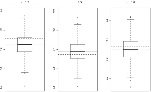
To verify the asymptotic behavior of our estimator under misspecification, we generate data from a Clayton copula ac-cording to DGP A.1 but in the estimation procedure we use a Gaussian copula. The “pseudo”-true quantile regression func-tion ismτ(x1;ρ∗)=−1(τ)
1−ρ∗2
+ρ∗x
1withρ∗=0.503
for the Clayton copula withα=1.Figure 1shows the boxplots
Table 1. The copula parameters and the marginal distributions for each subspecialized DGP.ν(·) is the cdf of a random variablet(ν)
DGP Copula parameter Marginal distribution mτ
A.1 α=1 Yi∼N(0,1), X1,i∼N(0,1) −1((1+(X1,i)−1(τ−1/2−1))−1) (Yi, X1,i)
A.2 α=0.5 Yi, Yi−1∼N(0,1) −1((1+(Yi−1)−1/2(τ−1/3−1))−2) (Yi, Yi−1)
B.1 ρ=0.6 Yi∼N(1,1), X1,i∼N(0,1) 1+0.8−1(τ)+0.6X1,i (Yi, X1,i)
B.2 =
⎛ ⎝
1 −0.5 0.9 −0.5 1 −0.4 0.9 −0.4 1
⎞
⎠ Yi∼U[0,1], X1,i∼N(0,1), (−0.17X1,i+0.83X2,i+0.41−1(τ))
X2,i∼N(0,1) (Yi, X1,i, X2,i)
B.3 =
⎛ ⎜ ⎜ ⎝
1 0.3 0.9 0.7 0.3 1 0.5 0.25 0.9 0.5 1 0.5 0.7 0.25 0.5 1
⎞ ⎟ ⎟
⎠ Yi∼U[0,1], X1,i∼N(0,1), (−0.20X1,i+0.83X2,i+0.33X3,i+0.27−1(τ))
X2,i∼N(0,1), X3,i∼N(0,1) (Yi, X1,i, X2,i, X3,i)
B.4 =
⎛ ⎜ ⎜ ⎝
1 0.6 0.3 0.4 0.6 1 0.5 0.2 0.3 0.5 1 0.6 0.4 0.2 0.6 1
⎞ ⎟ ⎟
⎠ Yi, Yi−1∼N(0,1), 0.65−1(4(Xi))−0.30Yi−1+ 0.44−1(
4(Xi−1))+0.72−1(τ) Xi, Xi−1∼t(4)
(Yi, Xi, Yi−1, Xi−1)
of the estimators ˆmτ(x1) obtained from 500 random samples of size 200. We see that the observed values are symmetrically distributed around the pseudo-true parametermτ(x1;ρ∗) instead of the true parametermτ(x1) as expected according to Theorem
3.1. The difference between these two quantities corresponds exactly to the asymptotic bias.
As for the time series setting, we generate 500 random sam-ples of size n=100 and 200 from DGPs A.2 and B.4. To
Table 2. ECPs of the confidence interval formτ(x) in the iid setting based on the asymptotic representation in Corollary 3.1
α=0.05 α=0.1
DGP x τ n=50 n=100 n=200 n=50 n=100 n=200
0.2 0.946 0.941 0.946 0.905 0.901 0.953
0.00 0.5 0.973 0.964 0.964 0.931 0.926 0.926
0.8 0.946 0.950 0.942 0.907 0.896 0.882
A.1
0.2 0.960 0.950 0.953 0.930 0.906 0.911
−1.64 0.5 0.959 0.959 0.960 0.915 0.923 0.918
0.8 0.924 0.938 0.938 0.881 0.894 0.892
0.2 0.947 0.951 0.948 0.898 0.895 0.901
0.00 0.5 0.956 0.946 0.958 0.913 0.899 0.911
0.8 0.952 0.948 0.962 0.912 0.888 0.918
B.1
0.2 0.846 0.879 0.891 0.792 0.825 0.829
−1.64 0.5 0.931 0.957 0.953 0.887 0.903 0.898
0.8 0.961 0.958 0.959 0.932 0.906 0.914
0.2 0.892 0.904 0.924 0.869 0.837 0.885
(0.00,0.00) 0.5 0.898 0.917 0.922 0.828 0.860 0.865
0.8 0.886 0.918 0.932 0.842 0.868 0.876
B.2 0.2 0.928 0.930 0.930 0.909 0.884 0.886
(1.53,1.53) 0.5 0.943 0.940 0.927 0.902 0.887 0.879
0.8 0.945 0.939 0.941 0.915 0.905 0.882
Table 3. ECPs of the confidence interval formτ(x) based on the true asymptotic representation and the bootstrap approach
α=0.05 α=0.1
DGP Method x τ n=50 n=100 n=200 n=50 n=100 n=200
B.2 TRUE 0.2 0.947 0.935 0.959 0.902 0.883 0.893
(0.00,0.00) 0.5 0.936 0.925 0.947 0.867 0.891 0.885
0.8 0.933 0.954 0.943 0.885 0.900 0.890
BT 0.2 0.950 0.946 0.948 0.896 0.906 0.906
(0.00,0.00) 0.5 0.950 0.948 0.952 0.884 0.890 0.898
0.8 0.932 0.940 0.960 0.876 0.886 0.878
compute a confidence interval formτ(x), we estimateσ2using the bootstrap described in Section3withB =200. We observe that the bootstrap seems to work reasonably well in terms of the ECP as shown inTable 4. The ECP whenα=0.1 seems to be somewhat higher than the nominal confidence level but gets closer to it as the sample size grows.
4.2 Comparison With Other Methods
In this section we compare our semiparametric estimator both with semiparametric and nonparametric competitors. We con-sider four estimators for comparison.
• mˆt c : our estimator when the true copula family is used. • mˆuc: our estimator when the copula density family is
adap-tively selected using the data (see the explanation below).
• mˆll: local linear estimator with the bandwidth selected by cross-validation based on the check-function.
• mˆsi : single index regression estimator based on a two stage estimation method; the single-index coefficients are first estimated by the method of Zhu, Huang, and Li (2012), and then the link function is estimated in the same way as for ˆmll.
In addition to this, we consider the nonlinear quantile re-gression estimator ˆmnl, which exploits the true link function as a reference case. We use the R packagequantregto calcu-late ˆmnl. Concerning the estimator ˆmuc, we use the simplified pair-copula decomposition of the copula density (R-vine) as in Noh, El Ghouch, and Bouezmarni (2013). The main idea of it is to decompose a multivariate copula to a cascade of bi-variate copulas so that we can take advantage of the relative
-1.6
-1.4
-1.2
-1.0
-0.8
τ =0.2
-0.8
-0.6
-0.4
-0.2
0.0
τ =0.5
0.0
0.2
0.4
0.6
τ =0.8
Figure 1. Boxplots of ˆmτ(x1) atx1=F1−1(0.2)= −0.8416 for different quantile levels (τ=0.2,0.5,and 0.8). The horizontal solid line representsmτ(x1;ρ∗) and the dotted line representsmτ(x1).
Table 4. ECPs of the confidence interval formτ(x) in the time series setting based on the bootstrap approach
α=0.05 α=0.1
DGP x τ n=100 n=200 n=100 n=200
A.2 0.2 0.948 0.958 0.926 0.920
0.00 0.5 0.962 0.954 0.934 0.924 0.8 0.948 0.956 0.914 0.906
B.4 0.2 0.952 0.952 0.924 0.902
(0.56,0.00,−0.27) 0.5 0.954 0.952 0.920 0.898 0.8 0.956 0.952 0.920 0.908
simplicity of bivariate copula selection and estimation. For de-tails, we refer to Aas et al. (2009), Brechmann (2010), Noh, El Ghouch, and Bouezmarni (2013), and references therein. Specifically, we choose one decomposition of the copula den-sity (among many R-vine structures) for the data, and then choose the pair-copulas independently among ten candidate cop-ulas: two are elliptical (Gaussian and Studentt) and eight are Archimedean (Clayton, Gumbel, Frank, Joe, Clayton-Gumbel, Joe-Gumbel, Joe-Clayton and Joe-Frank) using the R package VineCopula. As a selection criterion for bivariate copulas, we use the Akaike information criterion (AIC), which is shown to work in this context (see Dißmann et al.2013).
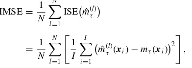
For comparison with other methods, we consider DGPs B.2 and B.3 to generate data. For performance evaluation of each method, we consider the empirical integrated mean squared error (IMSE), which is defined by
IMSE= 1
N
N
l=1
ISEmˆ(τl)
= 1
N
N
l=1
1
I
I
i=1
ˆ
m(τl)(xi)−mτ(xi)2
,
where {xi,i=1, . . . , I}is a fixed evaluation set which
cor-responds to a random sample of size I =500 generated from the distribution of X, ˆm(l)(·) is the estimated regression
func-tion from thelth data sample. As expected, the estimator ˆmnl performs best in both DGPs. Our estimator ˆmt c, which uses the information about the copula family, ranks the second. Addition-ally, even the estimator ˆmuc is a bit behind ˆmt c in performance due to the pair-copula selection step before the estimation, but it is still advantageous over the other semiparametric estimator
Table 5. 1000×IMSE for DGP B.2
N τ mˆt c mˆuc mˆnp mˆsi mˆnl
50 0.2 2.847 3.377 5.987 4.366 1.870 0.5 2.561 2.941 6.265 3.773 1.406 0.8 3.052 3.284 5.517 4.499 1.685 100 0.2 1.280 1.569 3.244 2.252 0.864 0.5 1.136 1.384 2.829 1.701 0.701 0.8 1.356 1.577 3.176 2.259 0.806 200 0.2 0.634 0.796 1.778 1.029 0.370 0.5 0.559 0.709 1.540 1.005 0.307 0.8 0.660 0.795 1.765 1.211 0.428
Table 6. 1000×IMSE for DGP B.3
N τ mˆt c mˆuc mˆnp mˆsi mˆnl
50 0.2 2.636 4.035 6.565 4.058 1.092 0.5 2.555 3.808 6.329 3.687 0.931 0.8 3.142 4.085 6.448 4.374 1.092 100 0.2 1.281 1.709 3.690 1.724 0.542 0.5 1.239 1.608 3.102 1.483 0.453 0.8 1.451 1.740 4.111 1.789 0.572 200 0.2 0.614 0.800 1.863 1.028 0.259 0.5 0.579 0.725 1.659 0.888 0.207 0.8 0.662 0.784 2.022 0.983 0.268
ˆ
msiand the nonparametric estimator ˆmnp. From this observation, we see that when the true DGP can be described using a certain copula which belongs to the copula family under consideration, which is the case here, our proposed methods can be a good choice in quantile regression. However, the performance of our estimators may depend on whether the true copula density fits into the copula family under our consideration or not. To see the impact of it, we consider an additional DGP.
• DGP CY =m(X1, X2, X3)+σ ǫ, whereǫ∼N(0,1) in-dependent ofX.
– m(X1, X2, X3)=(−0.3X1+0.9X2+0.3X3) where
is the cdf of the standard Cauchy distribution and
σ =0.1
– The resulting quantile regression function is
(−0.3X1+0.9X2+0.3X3)+0.1−1(τ).
– X=(X1, X2, X3)⊤is multivariate normal with mean0
and cov(Xj1, Xj2)=0.5|
j1−j2|.
Table 7shows the performance of each method. Note that since we have no knowledge about the true copula, the estima-tor ˆmt cis not available. In this case, as before the estimator ˆmnl performs best but the single-index estimator ranks the second in most cases. However, our estimator ˆmucstill shows comparable performance to ˆmsi and performs better than the nonparamet-ric estimator ˆmnp. This suggests that the copula family under consideration is flexible enough to approximate the true cop-ula density in a certain degree although it does not include the density. Additionally, it also implies that our method has the advantage over the classical single-index model and that it is more flexible and adapts better to different settings.
Table 7. 1000×IMSE for DGP C
N τ mˆuc mˆnp mˆsi mˆnl
50 0.2 4.106 4.167 3.609 0.419
0.5 3.835 3.904 3.046 0.300
0.8 4.449 4.918 4.445 0.427
100 0.2 2.422 3.286 2.393 0.190
0.5 2.037 3.116 2.174 0.146
0.8 2.416 3.800 2.597 0.193
200 0.2 1.562 2.206 1.881 0.093
0.5 1.286 1.975 1.157 0.087
0.8 1.539 2.226 1.409 0.091
0.00
0.05
0.10
0.15
Y
ahoo
0.00
0.02
0.04
0.06
0.08
0 100 200 300 400
Time
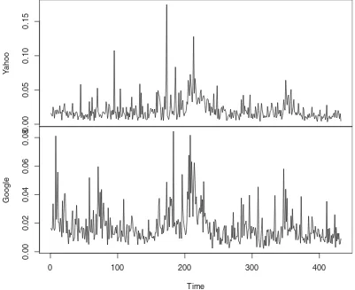
Figure 2. Plot of the historical volatilities for both companies.
5. EMPIRICAL APPLICATION
To illustrate the usefulness of our method, we analyze the historical volatilities of Yahoo({Yi}) and Google({Xi}) over a nine-year period (2004–2013, 2160 trading days). Every 5 trading days we compute the standard deviation of the log re-turns of each company and consider it as the historical volatil-ity of the period. The volatilities of both companies over the whole period are plotted inFigure 2(432 observations for each time series). When the volatility data for both companies in a certain length of period until a particular time point is given ({(Yi, Xi), i=1, . . . , n}), we consider a problem of predicting the volatility of the Yahoo company for the following period consisting of 5 trading days (Yn+1) using various copula-based
estimation models considered in this work. For prediction, we will use the conditional median estimate from each model. Here is the description of each model (M1–M6):
• (Yi, Yi−1)∼C(·,·;θ)⇒Yi|Yi−1
M1 -C: Gaussian copula, M2 -C: Studenttcopula
• (Yi, Xi)∼C(·,·;θ)⇒Yi|Xi
M3 -C: Gaussian copula, M4 -C: Studenttcopula
• (Yi, Xi, Yi−1, Xi−1)∼C(·,·,·,·;θ)⇒Yi|Xi, Yi−1, Xi−1
M5 -C: Gaussian copula, M6 -C: Studenttcopula
M1 and M2 only consider temporal dependence between the returns of the Yahoo company for prediction, whereas M5 and M6 consider both interdependence between the returns of the
two companies and temporal dependence in each company’s re-turns. Different from these models, M3 and M4 ignore temporal dependence and only focus on interdependence for prediction. To evaluate the performance of each model, we calculate the predicted value of Yn+1 repeatedly as we slide the time
win-dow of size n=50 (250 trading days = 1 year) by one week (5 trading days), and compare the predicted values with the observed ones. FromFigure 2, since it is clear that there exist both temporal dependence and interdependence, we expect that Models M5 and M6 considering both types of dependence will be better in prediction than the models considering just one of them. Before fitting the models, we checked whether the data of each company in each window satisfy at least stationarity using the Phillips–Perron unit root test (Phillips and Perron 1988). The tests never reject the stationarity assumption for both time series.
Table 8shows the prediction performance of each model mea-sured by the criterion (PRED=382k=1( ˆYk−Yk)2,kis an index for denoting evaluation points). As was expected, we observe that considering both dependence is better for prediction than only considering one kind of dependence regardless of the kind of copula used. This finding suggests that our extension to the
Table 8. PRED×105for each prediction method
M1 M2 M3 M4 M5 M6
PRED×105 24.659 24.610 21.811 21.131 21.634 21.107
multiple covariates case seems to be a useful contribution to the implementation of such idea. Additionally, from the fact that M3 and M4 are comparable with M5 and M6 in performance, we see that for these data the intercorrelation between two time series is a more important factor for prediction than the autocor-relation in the time series but this might not be the case in other data. Finally, one might think that since the current informa-tion (Xn+1) of the other company (Google), which might have
some link with the company of interest (Yahoo), is not always available for the prediction (ofYn+1), the model has some
lim-itation in practice. However, considering stocks of a company which has many branches overseas, such current information is available due to time difference.
6. CONCLUDING REMARKS
We proposed a new semiparametric conditional quantile es-timation method using copula-based multivariate models, espe-cially with the focus on the extension to the case of multiple covariates. We established the asymptotic properties of our esti-mator under general assumptions, which cover both the iid and the dependent case taking misspecification into account. Al-though we present some examples which fit into our theoretical framework, other interesting examples could be included in the proposed methodology. One example is higher-order Markov
β-mixing processes. For such data, the construction of a con-sistent copula parameter estimator, which is a key assumption for the validity of our copula-based method, needs more inves-tigation. It is not only a good future research topic, but also an important step to broaden the application of our work.
APPENDIX
In this appendix, we first prove a technical lemma and then present the proof of Theorem 3.1.
Lemma A.1. DefineAn(t)=i(ρτ(ǫi−t /√n)−ρτ(ǫi))c( ˆF0(Yi),
Using a first-order Taylor expansion, we have
A1,n=n−1/2 decompose further the termA11,nas
A11,n=n−1/2
Moreover, by Assumption (C0) and Donsker’s Theorem, see Theorem 7.2 in Rio (2000), supy|Fˆ0(y)−F0(y)| =Op(n−1/2). SoR1,n=op(1).
Now, we turn to the second termA12,n. Following the same argu-ments as forA11,n, by Assumptions (C1) and (C3), we have
A12,n=n−1/2
where, in the last equality, we used the weak law of large numbers and Assumption (C1).
Similarly, by Assumptions (C2) and (C3), the last termA13,ncan be expressed as
By Assumption (C0), using Hoeffding’s projection method and apply-ing Proposition 2 in Denker and Keller (1983), we get that
Vn=n−1
Using Assumption (C3)-(i), some easy calculations show that
λ(y)= −ψτ(y−mτ(x;θ∗))c(F0(y),F(x);θ∗)−
where, in the last equality, we used Assumption (C4). For the variance, observe that, O(n−1/2). Also, by the Cauchy–Schwarz’s inequality, we deduce that ifn−1≥kn,
for any integerkn→ ∞. On the other hand, by Assumption (C0), using Billingsley’s inequality, see for example, Lemma 3 in Doukhan (1994),
we also have that, for sufficiently largen,
n
By similar arguments, using Assumption (C0), (C3), and (C5), one can also show that
which concludes the proof of Lemma A.1.
Proof of Theorem 3.1.First, observe that, by definition,
arg min is a convex function of t. Thanks to Lemma A.1 and the quadratic approximation lemma (Basic Corollary in Hjort and Pollard 1993) withUn=Op(1), we have
which is the desired result.
ACKNOWLEDGMENTS
All the authors acknowledge financial support from IAP research network P7/06 of the Belgian Government (Belgian Science Policy). Additionally, H. Noh and I. Van Keilegom acknowledge financial support from the European Research Council under the European Community’s Seventh Frame-work Programme (FP7/2007–2013) / ERC grant agreement no. 203650, and A. El Ghouch and I. Van Keilegom acknowledge the support from the contract ‘Projet d’Actions de Recherche Concert´ees’ (ARC) 11/16-039 of the “Communaut´e franc¸aise de Belgique,” granted by the “Acad´emie universitaire Louvain.” Finally, the authors thank Fabian Y. R. P. Bocart for giving much help and sharing his insight concerning the application of our method to financial data.
[Received June 2013. Revised April 2014.]
REFERENCES
Aas, K., Czado, C., Frigessi, A., and Bakken, H. (2009), “Pair-Copula Construc-tions of Multiple Dependence,”Insurance: Mathematics and Economics, 44, 182–198. [174]
Bouy´e, E., and Salmon, M. (2009), “Dynamic Copula Quantile Regressions and Tail Area Dynamic Dependence in Forex Markets,”The European Journal of Finance, 15, 721–750. [167,168]
Brechmann, E. C. (2010), “Truncated and Simplified Regular Vines and Their Applications,” PhD thesis, Department of Mathematics, Technische Univer-sit¨at M¨unchen. [174]
Chen, X., and Fan, Y. (2006), “Estimation of Copula-Based Semipara-metric Time Series Models,” Journal of Econometrics, 130, 307–335. [167,168,169,170,171]
Chen, X., Koenker, R., and Xiao, Z. (2009), “Copula-Based Nonlinear Quantile Autoregression,”Econometrics Journal, 12, 50–67. [167,168]
Denker, M., and Keller, G. (1983), “OnU-Statistics and v. Mises’ Statistics for Weakly Dependent Processes,”Z. Wahrsch. Verw. Gebiete, 64, 505–522. [177]
Dißmann, J., Brechmann, E. C., Czado, C., and Kurowicka, D. (2013), “Se-lecting and Estimating Regular Vine Copulae and Application to Financial Returns,”Computational Statistics and Data Analysis, 59, 52–69. [174] Doukhan, P. (1994),Mixing: Properties and Examples(Lecture Notes in
Statis-tics), New York: Springer-Verlag. [177]
Genest, C., Ghoudi, K., and Rivest, L. (1995), “A Semiparametric Estimation Procedure of Dependence Parameters in Multivariate Families of Distribu-tions,”Biometrika, 82, 543–552. [169]
Hjort, N. L., and Pollard, D. (1993), “Asymptotics for Minimisers of Convex Processes,” Technical Report, Department of Statistics, Yale University. [177]
Ibragimov, R. (2009), “Copula-Based Characterizations for Higher Order Markov Processes,”Econometric Theory, 25, 819–846. [167,169]
Klaassen, C. A. J., and Wellner, J. A., (1997), “Efficient Estimation in the Bivariate Normal Copula Model: Normal Margins are Least Favourable,” Bernoulli, 3, 55–77. [169]
Koenker, R. (2005),Quantile Regression, Cambridge: Cambridge Universitey Press. [168]
Koenker, R., and Bassett, G. (1978), “Regression Quantiles,”Econometrica, 46, 33–50. [168]
Kojadinovic, I., and Yan, J. (2011), “A Goodness-of-fit Test for Multivariate Multiparameter Copulas Based on Multiplier Central Limit Theorems,” Statistics and Computing, 21, 17–30. [169]
Noh, H., El Ghouch, A., and Bouezmarni, T. (2013), “Copula-Based Regression Estimation and Inference,”Journal of the American Statistical Association, 108, 676–688. [168,169,173]
Phillips, P., and Perron, P. (1988), “Testing for a Unit Root in Time Series Regression,”Biometrika, 75, 335–346. [175]
R Development Core Team (2011), “R: A Language and Environment for Statis-tical Computing,” R Foundation for StatisStatis-tical Computing, Vienna, Austria. Available athttp://www.R-project.org/. [171]
R´emillard, B., Papageogiou, N., and Soustra, F. (2012), “Copula-Based Semi-parametric Models for Multivariate Time Series,”Journal of Multivariate Analysis, 110, 30–42. [167,169,170,171]
Rio, E. (2000),Th´eorie Asymptotique des Processus Al´eatoires Faiblement D´ependants, Heidelberg: Springer-Verlag. [169,170,176]
Silvapulle, P., Kim, G., and Silvapulle., M. J., (2004), “Robustness of a Semiparametric Estimator of a Copula,” inEconometric Society 2004 Aus-tralasian Meetings 317,Econometric Society. [169]
Silverman, B. W., and Young, G. A. (1987), “The Bootstrap: To Smooth or not to Smooth?”Biometrika, 74, 469–479. [171]
Sklar, M. (1959), “Fonctions de R´epartition `anDimensions et leurs Marges,” Publ. Inst. Statist. Univ. Paris, 8, 229–231. [168]
Tsukahara, H. (2005), “Semiparametric Estimation in Copula Models,” Cana-dian Journal of Statistics, 33, 357–375. [169]
Zhu, L., Huang, M., and Li, R. (2012), “Semiparametric Quantile Re-gression With High-Dimensional Covariates,” Statistica Sinica, 22, 1379–1401. [173]