ROBUST DECLINE CURVE ANALYSIS
Sutawanir Darwis, Budi Nurani Ruchjana, and Asep
Kurnia Permadi
Abstract. Empirical decline curve analysis of oil production data gives reasonable an-swer in hyperbolic type curves situations; however the methodology has limitations in fitting real historical production data in present of unusual observations due to the effect of the treatment to the well in order to increase production capacity. The development of robust least squares offers new possibilities in better fitting production data using decline curve analysis by down weighting the unusual observations. This paper proposes a robust least squares fitting lmRobMM approach to estimate the decline rate of daily production data and compares the results with reservoir simulation results. For case study, we use the oil production data at TBA Field West Java. The results demonstrated that the approach is suitable for decline curve fitting and offers a new insight in decline curve analysis in the present of unusual observations.
1. INTRODUCTION
Existing decline curve analysis are based on Arps equations(Arps, 1945), and there have been a great number of papers on this topic. Spivey (1986) presented an algo-rithm for hyperbolic decline curve fitting based on binomial and Taylor expansion. Fetkovich. Et al (1996) developed concepts for decline curve forecasting and pro-vided a theoretical basis for the Arps equations. Li and Horne (2003) developed a decline curve analysis based on fluid flow mechanism and discussed its application to Kern oil fields (Reyes, Li, Horne, 2004). Mattar and Anderson (2003) high-lighted the strengths and limitations of Arps decline analysis in a comprehensive methodology for analysis of production data. Decline curve analysis was used in evaluating well performance in multiwell system (Marhaendrajana and Blasingame,
Received 15-07-2008, Accepted 19-11-2009. 2000 Mathematics Subject Classification: 62G35.
Key words and Phrases: decline curve analysis, robust least squares.
2001). Cheng, Wang, McVay and Lee (2005) used stochastic approach to evaluate the uncertainty in reserve estimation based decline curve analysis. A stochastic reserve estimation using decline curve analysis using Monte Carlo simulation to obtained reserve distribution was discussed in Jochen and Spivey (1996).
Arps decline curve analysis is an empirical method and requires no knowl-edge of reservoir parameters. The application of the method involves estimating a parametric model to the historical production data using least squares method. There are many different curve fitting methods available, however there is no one clear method to handle unusual observations. The available methods leads to un-satisfactory results due to the influence of the unusual observation. This paper proposes a modification of Arps decline curve analysis using results from robust regression analysis where the unusual observations receives less weight compared with the other observations. The exponential decline curve is fitted using robust cube polynomial regression to obtain a better representation of the fluctuation of the historical production. The similar approach was developed for harmonic decline curve analysis. Inspired from growth curve modeling, a logistic decline curve is pro-posed to estimate the global trend and applied to the historical data. The robust trend curve fitting results Arps equations and logistic model are used to extrap-olated the future production decline and compared with the reservoir simulation results to evaluate the proposed approach.
2. ESTIMATING GLOBAL TREND
Management needs to reduce the risks associated with decision making, and one of the ways in which this can be done is by anticipating future well perfor-mance more clearly. Extrapolation of production history has long been considered the most accurate and defendable method of estimating remaining recoverable re-serve from a well and, in turn, a reservoir. The technique for relating production to time is known as decline curve analysis, and is a very useful tool for estimating future production. The decline curve is often used to determine the economic limit of a well, estimating the remaining reserves, and forecasting the present worth of the oil and gas reserves in the future. Three types of decline curves are considered, although only two of three techniques, namely, exponential and hyperbolic, com-monly occur in reservoirs. The hyperbolic decline model predicts a longer well life than is predicted by the exponential decline model. Also, the exponential forecast provides the lowest estimate of recoverable reserves. Experienced evaluators avoid extrapolating hyperbolic declines over long time periods, because they frequently result in unrealistically high reserve and value estimates. Arps [1] studied relation-ship between flow rate and time for producing wells. Assuming constant flowing pressure, he found relationship:
dq
dt =−Dq
(b+1)
(1)
The exponential decline curve corresponden tob=0, it has the solution:
q=q−Dt
0 (2)
whenq0 is the initial rate andDis a decline rate that is determined by fitting (2) to well or field data.
Harmonic decline curve occurs whenb=1, so the equation is:
q= q0
(1 +Dt (3)
Hyperbolic decline occurs when the decline rate is no longer constant. Com-pared to exponential decline, the following hyperbolic decline-curve equations esti-mate a longer production life of the well. Hyperbolic decline curve correspond to a value of b in the range 0<b<1. The rate solution has the form:
q= q0
(1 +bDt)1b
(4)
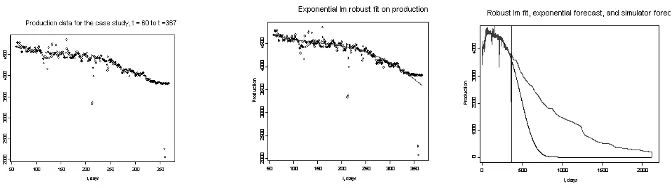
Figure 1 shows the plot of historical 367 daily production used as case study compared with the typical case of exponential and hyperbolic decline presented in Arps (1945). The plots indicate significant difference in the smoothness of the curve and fluctuation around global trend. Plot of 367 daily production data shows unusual observations due to the well treatment and a resistant statistical method is proposed to estimate the global trend and to reduce the influence of unusual observations.
Unusual observations are sample values which cause surprise in relation to the majority of the sample, and influence significantly to standard statistical techniques. The sample mean can be influenced completely whereas the median is little affected by moving any single value to±∞. The median is resistant whereas the mean is not. Many robust and resistant methods have been developed to be less sensitive to unusual observations. The basic treatment to unusual observations is by down weighting the observations. In a regression problem there are two possible sources of errors, the response and the corresponding predictors. Most robust methods in regression only consider the first and errors in predictors are ignored; and is known as the case for M estimators.
The plots above indicate significant difference in the smoothness of the curve. Plot of 367 daily production data shows unusual observations due to the well treat-ment and a resistant statistical method is proposed to estimate the global trend and to reduce the influence of unusual observations.
A great number of studies on production data are based on Arps decline curve analysis which represents the relationship between production and time during pseudosteady state period and is expressed in equation Arps (1945):
q= q0
(1 +Dt,0≤b≤1 (5)
where qt is the production at time t, q0 is the initial production at time t = 0,
Figure 1: (a) Historical 367 daily production data (b) Typical case of exponential decline, Arps (1945) (c) Typical case of hyperbolic decline
The equation summarizes the decline rates for exponential (b = 0), hyperbolic (0 < b < 1) and harmonic (b = 1). The linearization of exponential decline leads to linear regression of on t and can be estimated using standard least squares method. It is well known that the results of standard least squares are very sensitive to unusual observations. The results can be misleading.
This paper proposes a modification of least squares exponential decline by usinglmRobMM and a cube polynomial of t to reduce the influence of unusual pro-duction data and to capture the curvature of data fluctuation. lmRobMM performs high breakdown point and high efficiency regression. Robust regression models are useful for fitting linear relationships when the random variation in the data is not Gaussian (normal) or when the data contain significant outliers. In such sit-uations, standard linear regression may return inaccurate estimates. The robust MM regression method returns a model that is almost identical in structure to a standard linear regression model. This allows the production of familiar plots and summaries with a robust model.
The M estimator attempts to optimize the likelihood function. Similar idea was applied to harmonic decline curve; 1/qt is regressed with time t based on the equation 1/qt = (1 +Dt+At2+Bt3)/itq0 . Due to the similarity of de-cline curve to the growth modeling, a logistic curve was fitted to daily production
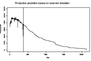
qt/q0=exp(−Dt+At2+Bt3)/(1 +exp(−Dt+At2+Bt3)) . Nls (nonlinear least squares) procedure was used to estimate and to evaluate the significance of the model parameters. The results from fitting the exponential decline, harmonic de-cline and logistic curve are compared to the reservoir simulation forecasting. The reservoir simulation results for t = 368 tot = 2127 days are based on fluid flow equations and implicit method using standard reservoir simulator software (Figure 2).
3. MAIN RESULT
Figure 2: Production prediction based on reservoir simulator
0.0012, and the fitted curve reproduces the curvature and the global trend of data fluctuation. However, there is a significance difference between predicted produc-tion with the reservoir simulator. The fitted model underestimates the simulator results. The display leads us to consider other models such as harmonic decline and logistic curve.
Figure 3: Robust least squares cube exponential decline rate, (a) The historical data used for model fitting (b) Global trend estimate using cube robust exponential decline (c) Comparison of the model prediction with reservoir simulator. The robust least squares underestimate the reservoir simulator
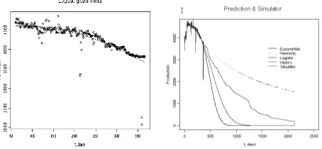
Figure 4: Robust harmonic decline curve, (a) The global trend estimate (b) The comparison with reservoir simulator, the harmonic decline over estimates the reser-voir simulator (c) Comparison of exponential and harmonic with reserreser-voir simula-tor, the reservoir simulator is in between these two curves.
Figure 5: Logistic decline curve, (a) Estimating global trend (b) Comparisons ex-ponential, harmonic, logistic and reservoir simulator. The logistic decline curve is close to the simulator compared with other models
4. CONCLUDING REMARKS
Acknowledgement. The authors thanks to the General Manager Deepwater Project, Chevron Indonesia Company, Chevron IndoAsia Business for financial support and Prof. Dr. J. Bruining also Dr. Rik Lopuhaa from TU Delft for a nice discussion.
REFERENCES
1. J.J. Arps, “Analysis of Decline Curves”,Trans AIME,160(1945), 228–247.
2. Y. Cheng, Y. Wang, McVay and W.J. Lee, “Practical Application of a Probabilistic Approach toEstimate Reserves Using Production Decline Data”,SPE95974, presented at Annual Technical Conference and Exhibition, Dallas Texas USA, (2005), 1–13. 3. M.J. Faddy and M.C. Jones, “Modelling and Analysis of Data that Exhibit Temporal
Decay”,Appl.Statist, C,48:2(1999), 229–237.
4. M.J. Fetkovitch, E. J. Fetkovitch, and M.D.Fetkovitch, “Useful Concepts for Decline Curve Forecasting, Reserve Estimation and Analysis”, SPE Reservoir Engi-neering (SPERE), (1996), 13–22.
5. N.F. Haavardsson, and A.B. Huseby, “Multisegment Production Profile - A Tool for Enhan- ced Total Value Chain Analysis”,Journal of Petroleum Science and Engineering ,58(2007), 325–338.
6. V.A. Jochen and J.P. Spivey, “Probabilistic Reserve Estimation Using Decline Curve Ana-lysis with the Bootstrap Method”, SPE36633, presented at SPE Annual and Technical Conference, Denver Colorado USA, (1996), 1–8.
Sutawanir Darwis: Statistics Research Division, Faculty of Mathematics and Natural Sciences, Institut Teknologi Bandung, Bandung, Indonesia.
E-mail:[email protected]
Budi Nurani Ruchjana: Department of Mathematics, Faculty of Mathematics and Natural Sciences, Universitas Padjadjaran, Bandung, Indonesia.
E-mail:[email protected]
Asep Kurnia Permadi: Reservoir Engineering Research Division, Faculty of Earth Sci-ences and Mining, Institut Teknologi Bandung, Bandung, Indonesia