SECOND ORDER LEAST SQUARE ESTIMATION ON ARCH(1) MODEL WITH BOX-COX TRANSFORMED DEPENDENT VARIABLE | Utami | Journal of the Indonesian Mathematical Society 166 455 1 PB

(1)

Vol. 19, No. 1 (2013), pp. 99–110.

SECOND ORDER LEAST SQUARE ESTIMATION

ON ARCH(1) MODEL WITH BOX-COX

TRANSFORMED DEPENDENT VARIABLE

Herni Utami

1

and Subanar

2

1_{Department of Mathematics Gadjah Mada University, Indonesia}

[email protected]

2_{Department of Mathematics Gadjah Mada University, Indonesia}

[email protected]

Abstract. Box-Cox transformation is often used to reduce heterogeneity and to achieve a symmetric distribution of response variable. In this paper, we estimate the parameters of Box-Cox transformed ARCH(1) model using second-order least square method and then we study the consistency and asymptotic normality for second-order least square (SLS) estimators. The SLS estimation was introduced by Wang (2003, 2004) to estimate the parameters of nonlinear regression models with independent and identically distributed errors.

Key words: Box-Cox transformation, second-order least square, ARCH model.

Abstrak. Transformasi Box-Cox sering digunakan untuk mengurangi heterogeni-tas dan mencapai distribusi simetris dari variabel respon. Pada paper ini dibahas estimasi parameter dari model ARCH(1) di mana variabel responnya ditransformasi Box-Cox dengan menggunakan metode estimasi second-order least square dan se-lanjutnya diteliti konsistensi dan normalitas asimtotik dari estimator second-order least square. Metode ini pertama kali diperkenalkan oleh Wang (2003, 2004) untuk mengestimasi parameter model regresi nonlinier yang variabel errornya berdistribusi identik dan independen.

Kata kunci: Transformasi Box-Cox, second-order least square, model ARCH

1. INTRODUCTION

Time series related to finance usually have three typical characteristics (Chan (2002)):

2000 Mathematics Subject Classification: 37M10.

(2)

(1) the unconditional distribution of financial time series such as stock price returns, has heavier tails than the normal distribution,

(2) the value of time series{Xt} is not correlated with each other, but {Xt2}

is strongly correlated with each other, (3) the volatility clustering.

One of the models that can be used to model the above conditions is Autoregressive Conditional Heteroscedastic (ARCH) model proposed by Engle (1982).

Two popular estimation methods for ARCH model are maximum likelihood and least square methods. Weiss (1986) discussed properties of maximum likeli-hood estimation and least square estimation of the parameters of both regression and ARCH equation. Basawa (1976) studied consistency and asymptotic normality for maximum likelihood estimators in the case where the observed random variables may be dependent and not identically distributed. The least square estimation pro-cedure for ARCH model is constructed in two stages. The first is to estimate the regression equation of the mean and the second is to estimate the regression equa-tion of variance. Therefore, using least square method for estimating the ARCH model will not obtain estimator for the mean and the variance regression simultane-ously. Wang and Leblanc (2008) estimated the parameters of nonlinear regression models with independent and identically distributed errors. We will propose sec-ond order least square (SLS) method to estimate parameters of ARCH model. The method does not require assumptions on the specific distribution of the errors and the estimators for mean and variance regression will be obtained simultaneously.

Box-Cox transformation can be used to reduce heterogeneity and achieve a symmetrical distribution of the response variable. Draper and Cox (1969) and Poiriers (1978) have shown that linearity, homoscedasticity, and normality cannot be done simultaneously with a certain Box-Cox transformation. Sarkar (2000) de-fined Box-Cox transformed ARCH model (BCARCH) and he considered maximum likelihood method to estimate parameters of BCARCH. Testing and estimation of BCARCH model are investigated and a Lagrange multiplier test is also developed to test Engle’s linear ARCH model against this wider class of models. In this paper, we propose second-order least square method to estimate parameters of BCARCH model.

The paper is organized as follows. In section 2, we describe Box-Cox trans-formed ARCH model. Estimation method is discussed in section 3. We developed method for testing power Box-Cox transformation in section 4. Finally, in section 5, Monte Carlo simulations of finite sample performance of the estimator is provided.

2. BOX-COX TRANSFORMED ARCH MODEL

(3)

predictor variables and response variable at the timetrespectively. The ARCH(R) models proposed in this paper is defined by

Yt|ℑt∼N(X′tβ, ht), (1)

whereℑtis the information set containing information about the process up to and

including timet−1 and

ht=α0+α1ε2t−1+· · ·+αRε2t−R. (2)

The error term, εt, has mean zero and varianceht which is split into a stochastic

pieceutand time-dependent variationhtcharacterizing the typical size of the term

so that εt = ut

√

ht. Coefficients α0 ≥ 0, αi > 0, so that conditional variance

is strictly positive, Xt is a k×1 vector of fixed observation at the time t on

p independent variables which may include this lagged value of the dependent variable,β′_{= (β}

1, β2, ..., βp) is a vector of associated regression coefficients.

Sarkar (2000) stated that the Box-Cox transformed ARCH(1) model is gen-eralization of the ARCH model and can be represented by

Y_t(λ)=X′

tβ+εt, (3)

ht=α0+α1ε2t−1, (4)

with

εt=ut

p

ht (5)

where 0≤α0,0< α1<1, (ut) is a sequence of iid random variables withE(ut) = 0

andE(u2

t) = 1. The Box-Cox transformed value of the (original) dependent variable

yt i.e.

y(_tλ)= (

Yλ t −1

/λ , λ6= 0 logYt , λ= 0

(6)

The transformation in equation (6) is valid only foryt>0 and, therefore,

modifica-tions have to be made for negative observation. Box and Cox proposed the shifted power transformation with the form

y(tλ)=

(

(yt+c) λ

−1

λ , λ6= 0

log(yt+c), λ= 0

(7)

where λ is the power transformation and c is chosen such that yt+c > 0 for

t = 1,2, ..., T. The λ is a parameter in this model, and the parameter indicates degree of nonlinearity in the data. The model reduces to the linear model when λ= 1. Hence, we develop test for the linear model by hypothesis H0 : λ= 1 vs

H1:λ6= 1.

The ARCH(1) model assume that Elog(α1ε2t)

< 0. The assumption is known to be necessary for stationarity, see Nelson (1990) for coefficient of condi-tional variance ofεton the GARCH (1,1) model is zero.

Conditional mean ofεtis given by

(4)

and conditional variance ofεtis

ht = E(ε2t|ℑt−1)

= α0+α1ε2t−1.

where α′ _{= (α}

0, α1) is a vector of parameters in the ARCH or variance equation.

The complete parameter vector for the model is θ′ _{= (λ, β}′_{, α}′_{). The parameter}

space as Θ⊂Rp+3_{is compact set that has at least one interior point.}

3. ESTIMATION

In this section, we briefly outline the estimation procedure for model (3) and (4) with the second-order least square estimation method proposed by Wang and Leblanc (2008), Abarin and Wang (2006). If θˆSLS is second-order least square

estimator for θ, then it is determined by minimizing the squared distance of the response variable to its first conditional moment and the square response variable to its second conditional moment of response variable:

QT(θ) =

1 T

T

X

t=1

ρ′

t(θ)Wtρt(θ) (9)

whereρt(θ) = (Yt(λ)−E(Ytλ|ℑt),(Yt(λ))2−E((Y

(λ)

t )2|ℑt))′ Wt=W(Xt) is weight

that is a 2x2 nonnegative definite matrix which may depend onXi.

The SLSE forθ can be represented ˆ

θSLS = arg min

θ QT(θ), (10) where θ _∈ Θ. In order to find θ which minimizes QT(θ) in equation (9), we

recommend using the algorithm proposed by Berndt et al (1974).

Lemma 3.1. Let εt be a ARCH(1) process,

εt=

p

htzt, zt∼IID(0, σ2), (11)

ht=α0+α1εt2−1, 0 ¡α1<1. (12)

Then{ε2

t} is an ergodic process.

Proof. _{Sequence (z}_t_{) is iid, so (z}_t_{) is stationary and ergodic. Repeatedly} substi-tuting forε2

t−1in equation (12), we have, fort≥1,

ht=α0

 

∞

X

j=0

αj1

j

Y

i=0

zt2−i



. (13)

Suppose

g(z0, z1, z2, ...) =α0

 

∞

X

j=0

αj1

j

Y

i=0

z2_t₋_i 

(5)

Let a sequence space S = {z= (zk) :zk∈R, k= 0,1,2, ...}. For z,y ∈ S and

Therefore, function g is continuous. By using ergodic theory, {ε2

t} is an ergodic

process.

Theorem 3.2. (Meyn and Tweedie (1993)) Function fn : Rd → R, n ∈ N are

continuous and they have partial derivative due to each variable. If there exists constantM such thatkfnk6M forn∈N andx∈Rdthen the family{fn, n∈N} Assumption 3E(ε4

t)<∞.

Theorem 3.3. Under assumption 1-3, the estimator SLSθˆ_SLS_−−→a.s θ0 asT → ∞.

Proof. _{By using ergodic theory,} _{_Q_T₍_θ₎_}_{is a ergodic process and we have}

(6)

The expected value ofρ′

By using inequality (15) and (16) we observe that

QT( ˆθSLS)−Q( ˆθSLS)6QT( ˆθSLS)−Q(θ0)6QT(θ0)−Q(θ0). (17)

Therefore from the above we have

QT(θ) is a continuous function on a compact set Θ and differentiable for every

(7)

such that k∇QT()k< M for everyT ∈N. By using theorem 3.2 we get{QT(θ)}

By inequality (18) we observe that

is a nonsingular matrix.

Assumption 5Ekqt(θ)|ℑt−1k4<∞whereqt(θ) =∂ρ

The method of the proof is to show that two conditions are satisfied.

(8)

Furthermore we can apply a Martingale central limit theorem (Billingsley, 1961 and 1965), so we obtain:

1

By the ergodic theory, we get 1

T Therefore, based on the equation (20), we obtain

1

Since Box-Cox transformed ARCH model is a generalization of the original ARCH model in which dependent variable has been transformed by the Box-Cox transformation, we need to test whether linear ARCH model provides an adequate description of the data or not. From section (3) we obtain that SLS estimators of Box-Cox transformed ARCH model are asymptotically normal in probability, so we can use z-test in the linearity testing. Consider testing a hypothesis about the first of coefficientθ. Theorem 3.3 implies that under theH0:λ= 1 (i.e., the linear

(9)

wherevar(ˆ_c λSLS) is the (1,1) element of the (P+ 3)×(P+ 3) matrix ˆB0−1Aˆ0Bˆ−01,

where

ˆ

B0= 1

T

X∂ρ′

t( ˆθ)

∂θ Wt

∂ρt( ˆθ)

∂θ′ ,

and

ˆ

A0= 1

T

X∂ρ′

t(θ0)

∂θ Wtρt(θ0)ρ

′

t(θ0)Wt

∂ρt(θ0)

∂θ′ .

The test statistics of the hypothesis is

t= p

T−(p+ 3)ˆλSLS−1

q c var(ˆλSLS)

→tT−(P+3).

5. SIMULATION

In order to study the performance of the SLS estimators ofθin finite samples, we simulated 100 series that is generated from ARCH(1) process with samples size T = 50,100,200,350:

Y_t(λ)=βY_t(₋λ₁)+εt, (21)

and

ht=α0+α1ε2t−1. (22)

where εt has mean zero and varianceht. We use values of the parameters of the

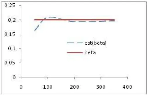
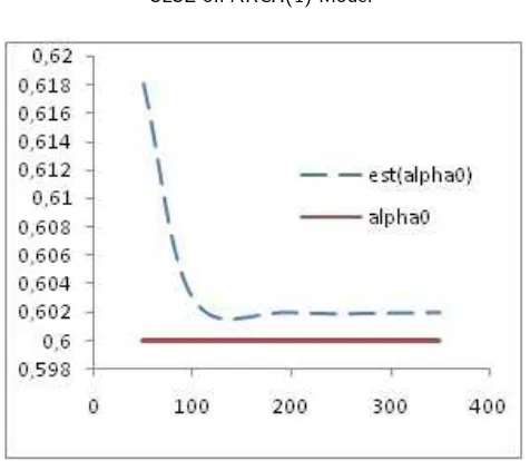
model in whichλ= 0.25, β = 0.2, α0= 0.60, and α1 = 0.15. Figure 1-4 show the

(10)

Table 1. SLS estimators of model (21) and (22)

λ= 0.25 β = 0.20 α0= 0.60 α1= 0.15

T λˆSLS MSE p-value βSLSˆ MSE αˆ0.SLS MSE αˆ1.SLS MSE

50 0.255 0.046 0.0005 0.163 0.024 0.618 0.032 0.063 0.058 100 0.253 0.018 0.0003 0.209 0.013 0.603 0.012 0.078 0.030 200 0.253 0.010 0.0003 0.194 0.007 0.602 0.008 0.109 0.029 350 0.252 0.006 0.0002 0.197 0.003 0.602 0.004 0.120 0.025

Figure 1. SLS estimation ofλ

(11)

Figure 3. SLS estimation ofα0

Figure 4. SLS estimation ofα1

REFERENCES

[1] Abarin, T., and Wang, L., ”Comparison GMM with Second-Order Least Square Estimation in Nonlinear Models”,Far East Journal of Theoritical Statistics,20(2)(2006), 179-196. [2] Alberola, R., ”Estimating Volatility Returns Using ARCH Models. An Empirical Case: The

Spanish Energy Market”,Lect. Econ,66(2006), 251-275.

(12)

[4] Berndt, E.K., Hall, R.E., Hausman, J.A., ”Estimation and Inference in Nonlinear Structural Models”,Ann. Econom. Social Measurement,4(1974), 653-665.

[5] Billingsley, P., ”The Lindeberg-Levy Theorem for Martingales”,Proceedings of The American Mathematical Society,12(5)(1961), 788-792.

[6] Billingsley, P.,Ergodic Theory and Information, Wiley, New York, 1965.

[7] Brockwell, P.J. and Davis, R.A.,Time Series: Theory and Methods, Springer-Verlag, Coro-lado, 1990.

[8] Capinski, M., Kopp, E.,Measure, Integral and Probability, Springer, New York, 2003. [9] Chan, N., H.,Time Series: Applications to Finance, John Wiley and Sons, Canada, 2002. [10] Draper, N.R., Cox, D.R., ”On Distributions and Their Trnsformation to Normality”,Royal

statistical Society- Series B 38(1969), 472-476.

[11] Engle, R.F., ”Autoregressive Conditional Heteroscedasticity with Estimates of The Variance of U.K. Inflation”,Econometrica,50(1982), 987-1008.

[12] Gao, S., He Yu, Chen, H., ”Wind Speed Forecast for Wind Farms Based on ARMA-ARCH Model”,IEEE (2009), 1-4.

[13] Hannan, E.J.,Multiple Time Series, Wiley, New York, 1970.

[14] Hayashi, F.,Econometric, Princeton University Press, United Kingdom, 2000.

[15] Hardle, W and Hafner, C.M., ”Discrete Time Option Pricing with Flexible Volatility Esti-mation”,Journal Finance and Stochaties,4(2)(2000), 189-207.

[16] Lamoureux, Christoper G., Lastrapes, William D., ”Heteroscedasticity in Stock Return Data: Volume Vesus GARCH Effect”,Journal of Finance,45(1)(1990), 221-229.

[17] Meyn, S.P., Tweedie, R.L.,Markov Chains and Stochastic Stability, Springer-Verlag, 1993. [18] Poiries, D.J., ”The Use of the Box-Cox Transformation in Limited Dependent Variable

Mod-els”,Journal of the American Statistical Association,73(1978), 284-287. [19] Rao, C.R.,Linear Statistical Inference and Its Applications, Wiley, Canada, 2002.

[20] Sarkar, N., ”ARCH model with Box-Cox Transformed Dependent Variable”,Statistics and Probability Letters,50(2000), 365-374.

[21] Wang, L., ”Estimation of Nonlinear Berkson-Type Measurement Error Models”, Statistica Sinica,13(2003), 1201-1210.

[22] Wang, L., ”Estimation of Nonlinear Models with Berkson Measurement Error”, Annals of Statistics,32(2004), 2559-2579.

[23] Wang, L., Leblanc, A., ”Second-Order Nonlinear Least Square Estimation”,Ann Inst Math 60(2008), 883-900.