BIOCLIME WP3 report Remote Sensing Solutions GmbH Final

(1)

Survey of biomass, carbon stocks, biodiversity, and assessment of the historic fire regime for integration into a forest monitoring system in South Sumatra, Indonesia.

Project number: 12.9013.9-001.00

Survey of biomass, carbon stocks, biodiversity, and assessment of the historic fire

regime for integration into a forest monitoring system in the Districts Musi Rawas,

Musi Rawas Utara, Musi Banyuasin and Banyuasin, South Sumatra, Indonesia

Work Package 3

Aboveground biomass and tree community composition modelling

Prepared by:

Uwe Ballhorn, Kristina Konecny, Peter Navratil, Juilson Jubanski, Florian Siegert RSS – Remote Sensing Solutions GmbH

Isarstraße 3 82065 Baierbrunn Germany

(2)

(3)

1

Table of Content

1. Introduction 2

2. Carbon and biodiversity plots 4

2.1. Inventory design 4

2.2. Aboveground biomass calculations 9

3. LiDAR data and aerial photos 13

3.1. LiDAR and aerial photo survey 13

3.2. LiDAR processing, filtering and interpolation 14

4. LiDAR based aboveground biomass model 17

4.1. Regression analysis and aboveground biomass model development 17

4.2. Determination of local aboveground biomass values 20

5. Analyses of tree community composition of lowland dipterocarp forests 23

5.1. Calculation of different LiDAR metrics for the biodiversity plots 23 5.2. Derivation of nMDS scores, biodiversity indices and pioneer/climax tree species ratio 23

5.3. LiDAR based tree community composition model 31

6. Conclusions 36

7. Outlook 36

Outputs / deliverables 37

References 38

Appendix A: Overview field plots 41

Appendix B: Overview biodiversity plots 47

Appendix C: Classification scheme 50

Appendix D: Overview LiDAR metrics lowland dipterocarp forest 52

Appendix E: Categorization of indetified tree species into pioneer or climax tree species. 54 Appendix F: Overview nMDS scores, biodiversity indices and ratios pioneer/climax tree species

(4)

Executive summary

With the Biodiversity and Climate Change Project (BIOCLIME), Germany supports Indonesia's efforts to reduce greenhouse gas emissions from the forestry sector, to conserve forest biodiversity of High Value Forest Ecosystems, maintain their Carbon stock storage capacities and to implement sustainable forest management for the benefit of the people. Germany's immediate contribution will focus on supporting the Province of South Sumatra to develop and implement a conservation and management concept to lower emissions from its forests, contributing to the GHG emission reduction goal Indonesia has committed itself until 2020.

One of the important steps to improve land-use planning, forest management and protection of nature is to base the planning and management of natural resources on accurate, reliable and consistent geographic information. In order to generate and analyze this information, a multi-purpose monitoring system is required.

The concept of the monitoring system consists of three components: historical, current and monitoring. This report presents the outcomes of the work package 3 “Aboveground biomass and tree community composition modelling” which is part of the current component.

The main objectives of WP 3 were:

 Filtering of the LiDAR 3D point clouds (provided by the project) into vegetation and non-vegetation points.

 Derive Digital Surface Models (DSM), Digital Terrain Models (DTM) and Canopy Height Models (CHM) from the airborne LiDAR data.

 Advice BIOCLIME in the collection of forest inventory data to calibrate the LiDAR derived aboveground biomass model.

 Derive an aboveground biomass model from the airborne LiDAR data (provided by the project) in combination with forest inventory data (provided by the project).

 Derive local aboveground biomass values for different vegetation classes from this LiDAR based aboveground biomass model.

 Derive a tree a community composition model of Lowland Dipterocarp Forest at various degradation stages from LiDAR data (provided by the project) in combination with tree species/genera diversity data collected in the field (provided by the project).

The results of the workpackage were a set of local aboveground biomass (AGB) values (Emission factors) derived from the LiDAR based aboveground biomass model for almost all identified vegetation cover classes. It was shown that aboveground biomass variability within vegetation classes can be very high (e.g. Primary Dryland Forest has a standard deviation for aboveground biomass of ±222.5 t/ha). Areas with the highest aboveground biomass (AGB) values were located within and around the Kerinci Seblat National Park.

(5)

1. Introduction

With the Biodiversity and Climate Change Project (BIOCLIME), Germany supports Indonesia's efforts to reduce greenhouse gas emissions from the forestry sector, to conserve forest biodiversity of High Value Forest Ecosystems, maintain their Carbon stock storage capacities and to implement sustainable forest management for the benefit of the people. Germany's immediate contribution will focus on supporting the Province of South Sumatra to develop and implement a conservation and management concept to lower emissions from its forests, contributing to the GHG emission reduction goal Indonesia has committed itself until 2020.

One of the important steps to improve land-use planning, forest management and protection of nature is to base the planning and management of natural resources on accurate, reliable and consistent geographic information. In order to generate and analyze this information, a multi-purpose monitoring system is required.

This system will provide a variety of information layers of different temporal and geographic scales:

 Information on actual land-use and the dynamics of land-use changes during the past decades is considered a key component of such a system. For South Sumatra, this data is already available from a previous assessment by the World Agroforestry Center (ICRAF).

 Accurate current information on forest types and forest status, in particular in terms of

aboveground biomass, carbon stock and biodiversity, derived from a combination of remote sensing and field techniques.

 Accurate information of the historic fire regime in the study area. Fire is considered one of the

key drivers shaping the landscape and influencing land cover change, biodiversity and carbon stocks. This information must be derived from historic satellite imagery.

 Indicators for biodiversity in different forest ecosystems and degradation stages.

The objective of the work conducted by Remote Sensing Solutions GmbH (RSS) was to support the goals of the BIOCLIME project by providing the required information on land use dynamics, forest types and status, biomass and biodiversity and the historic fire regime. The conducted work is based on a wide variety of remote sensing systems and analysis techniques, which were jointly implemented within the project, in order to produce a reliable information base able to fulfil the project’s and the partners’ requirements on the multi-purpose monitoring system.

This report presents the results of Work Package 3 (WP 3): Aboveground biomass and tree community composition modelling. The main objectives of WP 3 were:

 Filtering of the LiDAR 3D point clouds (provided by the project) into vegetation and non-vegetation points.

 Derive Digital Surface Models (DSM), Digital Terrain Models (DTM) and Canopy Height Models (CHM) from the airborne LiDAR data.

 Advice BIOCLIME in the collection of forest inventory data to calibrate the LiDAR derived aboveground biomass model.

(6)

 Deduce local aboveground biomass values for different vegetation classes from this LiDAR based aboveground biomass model.

 Derive a tree a community composition model of Lowland Dipterocarp Forest at various degradation stages from LiDAR data (provided by the project) in combination with tree species/genera diversity data collected in the field (provided by the project).

Figure 1 shows the flowchart of the activities carried out in Work Package 3 (WP 3).

Figure 1: Flow chart of the activities carried out in Work Package 3 (WP 3): Aboveground biomass and tree community composition modelling.

2. Carbon and biodiversity plots

2.1. Inventory design

(7)

112 carbon inventory plots where spatially shifted into the nearest LiDAR transect, consequently now not fitting into the systematic sampling design anymore.

The stratification of the forest areas was based on a combination forest type, altitude and soil type. The 112 carbon inventory plots were located in 10 different strata (see Table 1).

Table 1: Number of sample plots for each stratum.

Stratum1 Number of carbon inventory plots Primary Dryland Forest

(Hutan Lahan Kering Primer) 8 Secondary / Logged over Dryland Forest

(Hutan Lahan Kering Sekunder) 33 Primary Mangrove Forest

(Hutan Mangrove Primer) 13 Secondary / Logged over Mangrove Forest

(Hutan Mangrove Sekunder) 7 Primary Peat Swamp Forest

(Hutan Rawa Gambut Primer) 5 Secondary / Logged over Peat Swamp Forest

(Hutan Rawa Gambut Sekunder) 9

(8)

Figure 2: Layout of a rectangular nested carbon plot located in natural forests. Diameter at Breast Height (DBH) ranges in cm measured within the different rectangular nests (A, B, C, D and E) and the spatial orientation (N = North) are also given.

(9)

For all “in” trees within the carbon plots following parameters where recoded (an “in” tree was defined as a tree where the center of the stem at DBH is within the boundaries of the respective (sub)plot):

 Diameter at Breast Height(DBH) at 1.3 m above the ground (in centimeter)

 Total tree height(in meter) measured with a Haga instrument or a Suunto clinometer

 Tree species(scientific names in Latin): All “in” trees were identified up to the species level by a trained botanist. This was necessary to determine wood densities. Ideally it would be good to have an identification up to the species level as wood density can strongly vary within genus level. If it was not possible to identify up to the species level it was at least tried to record the genus or the family.

 Four dead wood classes (for the aboveground biomass estimates all dead trees were excluded):

 1 = many branches and twigs but without leaves

 2=large branches are still there but without a branch / small twigs and leaves

 3=almost no branches / twigs but still there are rods that may be broken

 4=just a broken rod topped resemble stumps

Additionally, to the carbon plots 58 so called biodiversity plots were recorded. The layout of these biodiversity plots is shown in Figure 4. The spatial locations of these biodiversity plots are exactly the same as the ones of the respective carbon plot.

(10)

For all “in” trees within the biodiversity plots following parameters where recoded (here also an “in” tree was defined as a tree where the center of the stem at DBH is within the boundaries of the respective (sub)plot):

 Diameter at Breast Height (DBH) at 1.3 m above the ground (in centimeter)

 Tree species (scientific names in Latin): All “in” trees were identified up to the species level by a trained botanist. This was necessary to determine wood densities. If it was not possible to identify up to the species level it was at least tried to record the genus or the family.

Table 2 gives an overview on how many carbon and biodiversity plots were recorded and whether they are located within LiDAR transects or not. As can be seen in Table 2, five plots were recorded after the fires of 2015. These plots have to be treated with care, as the LiDAR data was recorded before the fires of 2015.

Table 2: Overview carbon and biodiversity plots recorded and whether they are located within LiDAR transects or not.

Carbon plots Biodiversity plots Amount plots Amount plots within_{LiDAR transects}

X 54 (521₎ _{15 (13}1₎

X X 58 (551₎ _{48 (45}1₎

Sum 112 (1071₎ _{63 (58}1₎ 1_{Amount of plots after subtracting plots that were recorded after the fires of 2015}

Figure 5 displays the location of the recorded carbon and biodiversity plots within the four districts of Banyuasin, Musi Banyasin, Musi Rawas Utara and Musi Rawas. It also shows which of these carbon and biodiversity plots are located within a LiDAR transect.

Appendix A (Overview field plots) gives a detailed overview of all the 112 recorded plots and Appendix B (Overview biodiversity plots) gives and overview of the 58 recorded biodiversity plots. An in-depth explanation of the inventory design and collection is provided in the BIOCLIME GIZ Final Report: Panduan Survei Cadangan Karbon dan Keanekaragaman Hayati di Sumatera Selatan (Rusolono et al.

(11)

2.2. Aboveground biomass calculations

Rusolono et al. (2015) provide detailed procedures for analyzing the carbon stocks of the five carbon pools: aboveground biomass (AGB), belowground biomass (BGB), dead-wood, litter and soils. As the derived LiDAR AGB model is based on the estimated AGB from the carbon inventory plots only the derivation of AGB will be described in this report.

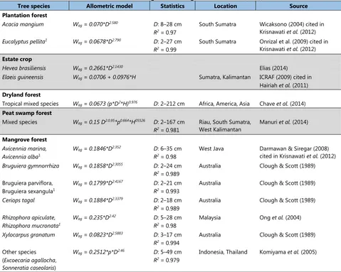
AGB consists of woody vegetation (saplings, poles and trees), non-woody vegetation (e.g. palms and bamboos) and understory vegetation. A detailed description of the analysis of woody vegetation biomass can be found in the BIOCLIME GIZ Final Report: Panduan Survei Cadangan Karbon dan Keanekaragaman Hayati di Sumatera Selatan (Rusolono et al. 2015). For each carbon inventory plot, the woody vegetation biomass of naturally grown trees species of saplings (DBH of 5-9 cm, within 0.0025 ha, subplot B), poles (DBH of 10-19 cm, within 0.01 ha, subplot C), small trees (DBH of 20-34 cm, within 0.04 ha, subplot D) and large tree (DBH ≥35 cm, within 0.1 ha, subplot E) as well as the woody vegetation biomass of planted tree species were estimated using allometric biomass models (Figure 2, Figure 3 and Table 3). Species-specific or genus-specific allometric biomass models were available only for some major tree species of plantation forest (i.e. Acacia mangium and Eucalyptus pellita), estate crops (i.e. Hevea brasiliensis and Elaesis guineensis) and mangrove species (i.e. Avicennia marina,

Avicennia alba, Bruguiera gymnorrhiza, Bruguiera parviflora, Bruguiera sexangula, Ceriops tagal,

Rhizophora apiculata, Rhizophora mucronata, Xylocarpus granatum, Excoecaria agallocha and

(12)

Manuri et al. (2014) and Komiyamaet al. (2005) were used to estimate tree AGB for dryland forests, peat swamp forests and other mangrove species (i.e. Excoecaria agallocha and Sonneratia caseolaris), respectively.

Table 3: Allometric biomass models for estimating tree aboveground biomass (AGB).

Tree species Allometric model Statistics Location Source Plantation forest

Acacia mangium Wag= 0.070*D2.580 D: 8–28 cm

R2_{= 0.97}

South Sumatra Wicaksono (2004) cited in Krisnawatiet al.(2012)

Eucalyptus pellita1 _W_ag_{= 0.0678*D}2.790 _D_{: 2–27 cm}

R2_{= 0.99}

South Sumatra Onrizal et al. (2009) cited in Krisnawatiet al.(2012) Estate crop

Hevea brasiliensis Wag= 0.2661*D2.1430 Elias (2014)

Elaeis guineensis Wag= 0.0706 + 0.0976*H Sumatra, Kalimantan ICRAF (2009) cited in

Hairiahet al.(2011) Dryland forest

Tropical mixed species Wag= 0.0673 (p*D2*H)0.976 D: 2–212 cm Africa, America, Asia Chaveet al.(2014)

Peat swamp forest

Mixed species Wag= 0.15 D2.0.95*p0.664*H05526 D: 2–167 cm

R2_{= 0.981}

Riau, South Sumatra,

West Kalimantan Manuriet al.(2014) Mangrove forest

Avicennia marina, Avicennia alba1

Wag= 0.1846*D2.352 D: 6–35 cm

R2_{= 0.98}

West Java Darmawan & Siregar (2008) cited in Krisnawatiet al.(2012)

Bruguiera gymnorrhiza Wag= 0.1858*D2.3055 D: 2–24 cm

R2_{= 0.989}

Xylocarpus granatum Wag= 0.0823*D2.5883 D: 3–17 cm

R2_{= 0.994}

Indonesia, Thailand Komiyamaet al.(2005)

Wag= aboveground biomass (kg),D= Diameter at Breast Height (DBH, cm),H= tree height (m),p= wood density (gram/cm3),R2=

coefficient of determination

1_{The aboveground biomass of these tree species were estimated using the available allometric models for similar tree species.}

(13)

of the total tree species), the allometric models used average wood density values that were derived from identified tree species in a particular stratum and location (Table 5).

Table 4: Diameter-height models for estimating tree height in some surveyed areas.

Stratum1 _Location _Model _Statistics

Secondary / Logged over Dryland Forest (Hutan Lahan Kering Sekunder / Bekas Tebangan)

PT REKI H=D/(0.7707+0.0195*D) nAIC= 168,= 1032.21,D= 5–104 cm,RMSE= 5.58,

(Hutan Mangrove Primer) TN Sembilang H= 28.1613*(1-exp(-D/27.0703))

n= 221,D= 5-77 cm,

AIC= 1098.86,RMSE= 2.89,

R2

adj= 0.750

D= Diameter at Breast Height (DBH, cm),H= tree height (m),n= number of samples,AIC= Akaike Information Criterion,RMSE= root mean square error,R2

adj= coefficient of determination adjusted

1_{in brackets Bahasa Indonesia}

Table 5: Average wood density for unidentified tree species.

Startum1 _Location Mean

(g/cm3₎ _(g/cmSt.dev.3₎2

Primary Dryland Forest

(Hutan Lahan Kering Primer) TN Kerinci Seblat 0.615 0.142 Secondary / Logged over Dryland Forest

(Hutan Lahan Kering Sekunder / Bekas Tebangan) PT REKI 0.594 0.143 Primary Mangrove Forest

(Hutan Mangrove Primer) Banyuasin 0.702 0.077 Secondary / Logged over Swamp Forest

(Hutan Rawa Sekunder / Bekas Tebangan) TN Sembilang 0.643 0.115

1_{in brackets Bahasa Indonesia} 2_{standard deviation}

Some carbon inventory plots (i.e. 7 plots or 4.9% of the total sample plots) also contained non-woody vegetation (i.e. bamboo, palm or rattan). The quantity of such non-woody vegetation, however, was very low with incomplete measurements of diameter or height, which resulted in difficulties when estimating their biomass. Therefore, the quantification of this insignificant non-woody biomass for these 7 sample plots was ignored.

The biomass of understory vegetation in each carbon inventory plot was estimated based on the field measurements and a laboratory analysis of the understory vegetation samples. The field measurements provided data on the sample’s fresh weight and total fresh weight of the understory vegetation, while the laboratory analysis provided data on the sample’s dry weight of the understory vegetation. The aboveground biomass of the understory vegetation was then calculated on the ratio of dry and fresh weights of the sample, which was then multiplied with the total fresh weight of the understory vegetation within a sample plot.

(14)

inventory is provided in the BIOCLIME GIZ Final Report: Cadangan Karbon Hutan dan Keanekaragaman Flora di Sumatera Selatan (Tiryanaet al.2015).

Table 6: Statistical results for the aboveground biomass (AGB) estimates for the different strata. Stratum1 Number of carbon

inventory plots Min AGB(t/ha)2 Max AGB_(t/ha)3 Mean AGB_(t/ha)4

(Hutan Lahan Kering Primer) 8 196.1 637.0 335.6 ±153.8 Secondary / Logged over Dryland Forest

(Hutan Lahan Kering Sekunder) 33 69.1 560.7 259.0 ±129.0 Primary Mangrove Forest

(Hutan Mangrove Primer) 13 159.8 531.3 304.7 ±98.8 Secondary / Logged over Mangrove Forest

(Hutan Mangrove Sekunder) 7 44.9 342.5 174.0 ±114.1 Primary Peat Swamp Forest

(Hutan Rawa Gambut Primer) 5 442.4 616.0 538.1 ±64.9 Secondary / Logged over Peat Swamp

Forest

(Hutan Rawa Gambut Sekunder)

9 114.9 414.0 207.1 ±89.9

Plantation Forest

(Hutan Tanaman) 8 5.4 133.8 59.9 ±43.7

Tree Crop Plantation

(Perkebunan) 15 3.4 211.6 62.2 ±55.4

Shrubs

(Semak Belukar) 6 8.7 127.2 59.6 ±54.0

Swamp Shrubs

(Semak Belukar Rawa) 8 1.3 105.5 55.5 ±41.5

Sum 112

1_{in brackets Bahasa Indonesia}

2_{Minimum aboveground biomass (AGB) in tons per hectare for the stratum} 3_{Maximum aboveground biomass (AGB) in tons per hectare for the stratum}

(15)

3. LiDAR data and aerial photos

3.1. LiDAR and aerial photo survey

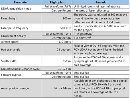
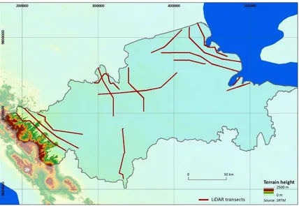
In October 2014 15 transects of LiDAR data and aerial photos were captured for an area of approximately 43,300 ha. LiDAR data was acquired in two modes (a) LiDAR full waveform mode + aerial photos with an overlap of 60% and (b) LiDAR discrete return mode + aerial photo overlap 80%. Table 7 displays the technical specification of this LiDAR and aerial photo survey. A more detailed description of the survey can be found in the report of the surveying company PT Asi Pudjiastuti Geosurvey (PT Asi Pudjiastuti Geosurvey 2014).

Table 7: Technical specifications of the LiDAR and aerial photo survey (PT Asi Pudjiastuti Geosurvey 2014).

Parameter Flight plan Remark

LiDAR acquisition mode Full Waveform (FWF) Unlimited returns of laser reflectance_{Discrete Return 4 returns of laser reflectance}

Flying height 800 m

The survey was conducted at 800 m above ground level to get the accurate laser reflectance and minimize cloud cover. Laser pulse frequency 500 KHz Product specification in ALS70 Leica used_{for the project.} LiDAR point density Full Waveform (FWF) 8-15 points/m2

Discrete Return 6-8 points/m2

Aircraft speed 110 knots

Half scan angle 28 degrees

Field of view (FOV) 56 degrees. With this FOV LiDAR coverage will be embedded with aerial photo coverage.

Swath width 851 m

A scan angle (FOV) of 56 degrees and a flying height of 800 m will provide 851 m area coverage

Ground Sample Distance (GSD) 10-12.5 m

Forward overlap Full Waveform (FWF) 60% overlap Discrete Return 80% overlap

Aerial photo coverage 86 m x 644 m

Acquisition of aerial photos using a digital camera: Leica RCD 30 with 6 µm pixel resolution, with a GSD of 10 cm per pixel will results in a coverage of 860 m x 644 m.

(16)

Figure 6: Location of the approximately 43,300 ha of LiDAR transects captured within the BIOCLIME study area.

3.2. LiDAR processing, filtering and interpolation

(17)

(18)

Figure 8: Location of the LiDAR 3D points clouds shown in Figure 7 within the BIOCLIME study area and the corresponding LiDAR derived Canopy Height Models (CHM).

Products derived from these LiDAR 3D point clouds include a Digital Surface Model (DSM) which represents the elevation of the vegetation canopy, a Digital Terrain Model (DTM) which represents the ground elevation, and a Canopy Height Model (CHM) which is generated by subtraction of the DTM from the DSM and represents the vegetation height. The LiDAR data was processed using the Trimble Inpho software package.

A crucial step within the DTM generation is the LiDAR filtering. A hierarchic robust filter was applied to the LiDAR 3D point clouds, separating the ground and non-ground (vegetation) points (Pfeifer et al.

(19)

Figure 9: Example from the LiDAR products generated for the BIOCLIME study area. Shown are examples for the Digital Terrain Model (DTM; 1 m spatial resolution) the Digital Surface Model (DSM; 1 m spatial resolution) and the Canopy Height Model (CHM; 1 m spatial resolution). Also shown are the position of the 63 carbon inventory plots that are located within the LiDAR transects.

4. LiDAR based aboveground biomass model

4.1. Regression analysis and aboveground biomass model development

(20)

The commonly used power function resulted in significant overestimations in the higher biomass range within our study areas. For this reason, a more appropriate aboveground regression model was implemented, which is a combination of a power function (in the lower biomass range up to a certain threshold QMCH0; the example here uses QMCH but the same would be done with CH) and a linear

function (in the higher biomass range) (Englhartet al. 2013). The threshold of QMCH0 was determined

by increasing the value of QMCH0 in steps of 0.001 m through identifying the lowest Root Mean

Square Error (RMSE). The linear function is the tangent through QMCH0 and was calculated on the

basis of the first derivative of the power function:

Where QMCH is the quadratic Mean Canopy Height (the example here uses QMCH but the same would be done with CH), QMCH0is the threshold of function change and a, b are coefficients. Next the

aboveground regression with the highest coefficient of determination (r2_{) based on the QMCH or the}

CH was chosen.

Of the 63 carbon plots that were located within the LiDAR transects 52 plots (after removal of obvious outliers) were used for calibration. The model based on QMCH achieved better results as the one based on CH. Figure 10 displays the results of the QMCH based LiDAR regression model.

Figure 10: Predictive aboveground biomass (AGB) model used for the BIOCLIME study area based on carbon plot data and airborne LiDAR data. The Quadratic Mean Canopy Height (QMCH) was chosen as it had a higher coefficient of determination (r2_{) as the Centroid Height (CH) based model.}

(21)

Next a spatially explicit aboveground biomass model was created by applying the above described regression model. The LiDAR based aboveground biomass model was created at 5 m spatial resolution i.e. each pixel represents an area of 0.1 ha. For ease of interpretation the cell values were scaled to represent aboveground biomass in tons per hectare. Figure 11 displays the final LiDAR based aboveground biomass model and gives examples of Lowland Dipterocarp Forest, Peat Swamp Forest and Mangrove.

(22)

4.2. Determination of local aboveground biomass values

In order to derive local aboveground biomass values for the different land cover classes, the spatial aboveground biomass model was overlaid with the land cover classification from Work Package 2 (WP 2) and zonal statistics (minimum, maximum, mean and standard deviation) on aboveground biomass were extracted for the respective land cover class (see Figure 12). To avoid possible misclassifications at land cover class borders a buffer of 60 m was excluded from the zonal statistics.

Figure 12: Schematic representation of the extraction of zonal statistics. The aboveground biomass (AGB) model is overlaid with the land cover classification (from Work Package 2) and zonal statistics on aboveground biomass are extracted for the respective land cover class. In this example the mean AGB in tons per hectare (t/ha) for the respective land cover class (LCC) is shown.

Zonal statistics were extracted for the BAPLAN and BAPLAN enhanced land cover classes (see Appendix C). Table 8 and Table 9 display these derived local aboveground biomass values. For the land cover classes not present in the aboveground biomass model missing values were estimated based on existing values or missing values were based on values from scientific literature.

(23)

Table 8: Local aboveground biomass values derived from zonal statistics of the LiDAR aboveground biomass model for the different forest type / land cover classes based on BAPLAN.

Forest type / land cover BAPLAN1 _{Mean AGB (t/ha)}2 _{SD (t/ha)}3 _{Min AGB (t/ha)}4 _{Max AGB (t/ha)}5 _{Area (ha)}6

Primary Dryland Forest 586 ±157.8 38.2 1,404.8 2,285.2

Secondary / Logged over Dryland Forest 305 ±158.8 0.0 1,206.5 5,685.3

Primary Swamp Forest 279 ±97.8 4.7 709.0 1,806.5

Secondary / Logged over Swamp Forest 108 ±78.6 0.2 505.4 1,363.3

Primary Mangrove Forest 249 ±106.7 0.0 668.8 4,031.9

Secondary / Logged over Mangrove Forest 72 ±34.4 14.0 284.4 71.7 Mixed Dryland Agriculture / Mixed Garden 144 ±100.2 0.0 712.3 1,883.0

Tree Crop Plantation 49 ±63.2 0.0 428.9 442.2

Plantation Forest 64 ±45.8 0.0 406.5 517.5

Scrub 39 ±57.3 0.0 762.4 964.6

Swamp Scrub 15 ±19.1 0.2 123.1 3.3

Rice Field7 ₁₀ _- _- _-

-Dryland Agriculture 48 ±64.1 0.0 487.0 126.3

Grass8 ₆ _- _- _-

-Open Land9 _{(0) 29} _±75.7 _0.0 _749.0 _13.4

Settlement / Developed Land9 _{(0) 23} _±14.8 _0.2 _81.8 _1.3

Water Body9 _{(0) 164} _±68.8 _1.1 _469.3 _83.2

Swamp 22 ±20.7 0.3 80.8 1.3

Embankment9 _{(0) 2} _±4.1 _0.0 _25.1 _9.5

1_{Forest type/land cover class BAPLAN classification system}

2_{Mean aboveground biomass (AGB) in tons per hectare for the forest type/land cover class} 3_{Standard deviation (SD) in tons per hectare for the forest type/land cover class}

4_{Minimum aboveground biomass (AGB) in tons per hectare for the forest type/land cover class} 5_{Maximum aboveground biomass (AGB) in tons per hectare for the forest type/land cover class} 6_{Area in hectare from which zonal statistics are based on}

7_{Value for Rice Field from scientific literature (Confalonieri}_{et al.}₂₀₀₉₎ 8_{Value for Grass from scientific literature (IPCC 2006)}

(24)

Table 9: Local aboveground biomass values derived from zonal statistics of the LiDAR aboveground biomass model for the different forest type / land cover classes based on BAPLAN enhanced.

Forest type / land cover BAPLAN enhanced1 Mean AGB

(t/ha)2 SD (t/ha)3 Min AGB_(t/ha)4 Max AGB_(t/ha)5 Area (ha)6

High-density Upper Montane Forest7 ₃₀₄ _- _- _-

-Medium-density Upper Montane Forest8 ₂₂₈ _- _- _-

-Low-density Upper Montane Forest7 ₁₉₂ _- _- _-

-High-density Lower Montane Forest 653 ±129.0 229.6 1106.7 52.0

Medium-density Lower Montane Forest 529 ±77.3 358.3 789.0 5.5

Low-density Lower Montane Forest7 ₂₆₈ _- _- _-

-High-density Lowland Dipterocarp Forest 584 ±158.0 38.2 1404.8 2,233.2 Medium-density Lowland Dipterocarp Forest 340 ±152.7 0.0 1206.5 4,536.6

Low-density Lowland Dipterocarp Forest 166 ±92.8 0.3 986.8 1,143.2

High-density Peat Swamp Forest 287 ±100.0 5.3 709.0 1,430.7

Medium-density Peat Swamp Forest8 ₂₁₆ _- _- _-

-Low-density (Regrowing) Peat Swamp Forest 110 ±86.6 0.9 505.4 590.7

Permanently Inundated Peat Swamp Forest 244 ±86.9 4.7 568.1 301.1

High-density Swamp Forest

(incl. Back- and Freshwater Swamp) 256 ±52.5 13.5 399.0 74.8

Medium-density Swamp Forest

(incl. Back- and Freshwater Swamp)8 192 - - -

-Low-density (Regrowing) Swamp Forest

(incl. Back- and Freshwater Swamp) 107 ±71.9 0.2 444.4 772.6

Heath Forest7 ₂₂₄ _- _- _-

-Mangrove 1 268 ±99.8 0.0 668.8 3,473.1

Mangrove 2 200 ±95.7 26.2 515.3 86.0

Nipah Palm 115 ±37.8 0.9 456.6 472.8

Degraded Mangrove 74 ±34.9 14.0 218.9 57.8

Young Mangrove 65 ±31.0 17.5 284.4 13.9

Dryland Agriculture mixed with Scrub 38 ±47.1 0.0 508.8 414.2

Rubber Agroforestry 174 ±90.4 0.0 712.3 1,468.8

Oil Palm Plantation 27 ±42.2 0.0 336.0 304.2

Coconut Plantation 58 ±27.1 2.5 132.2 94.1

Rubber Plantation 185 ±66.6 0.6 428.9 43.9

Acacia Plantation 64 ±48.6 0.0 236.6 360.2

Industrial Forest 63 ±38.7 0.5 406.5 157.3

Scrubland 39 ±57.3 0.0 762.4 964.6

Swamp Scrub 15 ±19.1 0.2 123.1 3.3

Rice Field9 ₁₀ _- _- _-

-Dryland Agriculture 48 ±64.1 0.0 487.0 126.3

Grassland10 ₆ _- _- _-

-Bare Area11 _{(0) 29} _±75.7 _0.0 _749.0 _13.4

Settlement11 _{(0) 10} _±14.2 _0.2 _81.8 _0.4

Road11 _{(0) 29} _±10.6 _0.3 _49.6 _0.9

Water11 _{(0) 164} _±68.8 _1.1 _469.3 _83.2

Wetland 22 ±20.7 0.3 80.8 1.3

Aquaculture11 _{(0) 2} _±4.1 _0.0 _25.1 _9.5

1_{Forest type/land cover class BAPLAN enhanced classification system} 7_{Values from FORCLIME (Navratil 2012)}

2_{Mean aboveground biomass (AGB) in tons per hectare for the forest type/land cover class} 8_{Calculated as 75% of respective high density class}

3_{Standard deviation (SD) in tons per hectare for the forest type/land cover class} 9_{Value for Rice Field from scientific literature (Confalonieri}_{et al.}₂₀₀₉₎ 4_{Minimum aboveground biomass (AGB) in tons per hectare for the forest type/land cover class} 10_{Value for Grass from scientific literature (IPCC 2006)}

5_{Maximum aboveground biomass (AGB) in tons per hectare for the forest type/land cover class} 11_{Value in brackets was finally used as local aboveground biomass value as} the

(25)

5. Analyses of tree community composition of lowland dipterocarp forests

5.1. Calculation of different LiDAR metrics for the biodiversity plots

From the airborne LiDAR data following 19 LiDAR metrics per biodiversity plot located within a LiDAR transect (n = 28) were derived (Table 10).

Table 10: LiDAR metrics derived for each biomass plot located within the LiDAR transects (n = 28). Also shown in the respective abbreviation and which software method was used to derive them.

LiDAR metric Abbreviation Software / method used

Quadratic Mean Canopy Height (QMCH) QMCH in house script

Centroid Height (CH) CH in house script

Maximum height Max LASTools1

Mean height Mean LASTools1

Standard deviation height SD LASTools1

Forest cover at 1 m height cov 1m LASTools1

5th_{height percentile} _{p 5}th _LASTools1

1_{https://rapidlasso.com/lastools/}

Appendix D displays these LiDAR metrics for all the biodiversity plots located in lowland dipterocarp forest (all further tree community composition analyses are for lowland dipterocarp forest only). These LiDAR metrics were then correlated to the nMDS scores, biodiversity indices and ratios between pioneer and climax tree species derived in Chapter 5.2 (Derivation of nMDS scores, biodiversity indices and pioneer/climax tree species ratio) in order to derive a predictive LiDAR based tree community composition model (see Chapter 5.3 LiDAR based tree community composition model).

5.2. Derivation of nMDS scores, biodiversity indices and pioneer/climax tree

species ratio

(26)

species could be identified, where only genus, family, common name was known and unidentified trees.

Table 11: Absolute and percentage of tree identification (species, only genus, only family, only common name and unidentified) within the biodiversity plots.

All trees

recorded identifiedSpecies Only genusidentified Only familyidentified Only commonname Unidentified Absolute

number 2733 2408 284 15 4 22

Percent (%) 100% 88% 10% 1% 0% 1%

All further analyses on tree community composition were conducted for lowland dipterocarp forest only. Mangrove was excluded as the variety of different tree species in the observed mangroves was very low (only up to six different tree species). Peat swamp forest was excluded because only three biodiversity plots were available and all were recorded after the fires of 2015.

Because some trees could not be identified to the species level all analyses on tree community composition are based on the genus level. Imaiat al.(2014) showed that results on the genus level are highly correlated with those at the species level.

The similarity in tree community composition for the different lowland dipterocarp forest density classes (low, medium and high) was not only assessed for the stratification of the biodiversity plots based on the satellite classification derived from Work Package 2 (WP 2) but also for a stratification based on the forest cover at 10 meter height above the ground (LiDAR metric was derived in the previous chapter). The thresholds for the two additional stratifications are shown in Table 12.

Table 12: Additional stratification of the biodiversity plots based on the forest cover at 10 meter height above the ground (LiDAR metric was derived in Chapter 5.1).

Lowland dipterocarp forest density class Stratification thresholds

Forest cover at 10 m height above ground (%) Low-density Lowland Dipterocarp Forest 0-<40

Medium-density Lowland Dipterocarp Forest 40≤-<80 High-density Lowland Dipterocarp Forest 80≤

(27)

Nonmetric multidimensional scaling (nMDS)

To assess the effects of different degradation levels on forest biodiversity the degree of similarity in tree community composition has gained increasing attention (Ioki et al.2016, Barlow et al.2007, Imai

et al. 2012, Imai et al. 2014, Magurran and McGill 2011, Su et al. 2004, Ding et al. 2012). Nonmetric multidimensional scaling (nMDS) was applied to assess the differences in tree community composition among the biodiversity plots. The number of trees of each genus within the 38 biodiversity plots located in lowland dipterocarp forest was used as input to the Bray-Curtis similarity index to calculate the nMDS scores of axis 1 and axis 2. Figure 13 and Figure 14 display the resulting scatter plots from the nMDS calculation for the two density stratifications (base on the satellite classification of Work Package 2 and the forest cover at 10 m height). In both scatterplots the nMDS axis 1 scores of High-density Lowland Dipterocarp Forest and Low-High-density Lowland Dipterocarp Forest are mostly located at the opposite ends of nMDS axis 1 indicating a difference in tree community composition of these two classes. The nMDS axis 1 scores of Medium-density Lowland Dipterocarp Forest is mostly located between the scores of the two other density classes.

(28)

(29)

(30)

Simpson index 1-D

The Simpson index 1-D was calculated for each biodiversity plot. This index measures ‘evenness’ of the community from 0 (one taxon dominates the community completely) to 1 (all taxa are equally present).

whereniis the number of individuals of taxoni.

Shannon index (entropy)

The Shannon index (entropy) was calculated for each biodiversity plot. The Shannon index (entropy) is a diversity index, taking into account the number of individuals as well as the number of taxa. The index increases as both the ‘richness’ and the ‘evenness’ of the community increases. It varies from 0 for communities with only a single taxon to high values for communities with many taxa, each with few individuals.

whereniis the number of individuals of taxoni.

In most ecological studies the values are generally between 1.5 and 3.5 and the index is rarely greater than 4.

Margalef’s richness index

The Margalef’s ‘richness’ index was calculated for each biodiversity plot. This index is a ‘richness’ index that attempts to compensate for sampling effects such as sample size. The higher the index the higher the ‘richness’.

Equitability

Equitability was calculated for each biodiversity plot. Equitability is the Shannon diversity divided by the logarithm of number of taxa. This measures the ‘evenness’ with which individuals are divided among the taxa present. The higher the index the higher the ‘evenness’.

Ratio pioneer/climax tree species

(31)

categorized as pioneer and climax species were treated as climax species. An overview of this categorization is shown in Appendix E. The ratios calculated for the respective biodiversity plots lie between 0 (only climax species) and 1 (only pioneer species).

Appendix F gives an overview of the two forest stratifications (satellite classification and forest cover at 10 m height), the nMDS scores of axes 1 and 2 for the respective forest stratifications, the four biodiversity indices and the ratio between pioneer and climax tree species.

As there was no statistical significant correlation between the forest density classes and the nMDS scores of axis 2, only scores from axis 1 very implemented in subsequent analyses.

Table 13 displays the descriptive statistics on the nMDS axis 1 scores, the four biodiversity indicators and the ration between pioneer and climax tree species for the different Lowland Dipterocarp Forest density classes (Low, Medium and High). The stratification of the density classes is based on the forest cover at 10 m height. These results show that there is a gradient in the mean nMDS axis 1 scores where Low-density Lowland Dipterocarp Forest with -0.214 had the lowest mean and High-density Lowland Dipterocarp Forest the highest with 0.109. Looking at the biodiversity indicators the two indices for ‘richness/diversity’ (Shannon index and Margelef’s index) also had a similar gradient where the Low-density Lowland Dipterocarp Forest had the lowest and the High-density Lowland Dipterocarp Forest had the highest mean values indicating that High-density Lowland Dipterocarp Forest has the highest biodiversity. Also the other two biodiversity indicators for ‘evenness’ (Simpson index 1-D and Equitability) have a similar gradient which indicates that the High-density Lowland Dipterocarp Forest has the highest ‘evenness’ (all taxa are more equally present). With regard to the ratio between pioneer and climax tree species also a gradient could be observed where Low-density Lowland Dipterocarp Forest with a mean of 0.504 had the highest and High-density Lowland Dipterocarp Forest with a mean of 0.097 had the lowest value. This indicates that Low-density Lowland Dipterocarp Forest compared to High-density Lowland Dipterocarp Forest feature proportionally more pioneer tree species and vice versa.

(32)

Table 13: Descriptive statistics on the nMDS axis 1 scores and the four biodiversity indicators for the different Lowland Dipterocarp Forest density classes: Low, Medium and High. The density classes are based on the forest cover at 10 m height stratification.

(33)

between the means of the different density classes (Low, Medium and High) for the nMDS axis 1 scores, Shannon index and Margelef’s index. Further, for all these three indicators the Tukey’s pairwise post-hoc test showed there was a statistical significant (p< 0.05) difference between the density pairs Low vs Medium and Low vs High but not for Medium vs High. For the Simpson index 1-D, the Equitability and the ratio between pioneer and climax tree species no statement on the difference between the density classes could be made as one or more of the density groups was not normally distributed, which is a requirement for a One-Way ANOVA.

Table 14: Results of the statistical analyses comparing the different Lowland Dipterocarp Forest density classes: Low, Medium and High. The density classes are based on the forest cover at 10 m height stratification. Numbers in the cells represent the p values. Cells in green show that the respective test results are positive and cells in red that the respective test results are negative. Shaded cells indicate that here a One-Way ANOVA could not be conducted as one or more of the density groups was not normally distributed. (p< 0.05;n= 28)

nMDS axis 1 Simpson index 1-D Shannon index Test normal

distribution1

Low Medium High Low Medium High Low Medium High

0.477 0.752 0.896 0.079 0.000 0.033 0.187 0.097 0.574

One-way ANOVA2 _0.000 _0.000 _0.000

Tukey’s pairwise3

Medium High Medium High Medium High Low 0.003 0.000 0.000 0.000 0.001 0.000

Medium X 0.161 X 0.716 X 0.445

Margelef’s index Equitability Ratio pioneer/climax_{tree species}

Test normal distribution1

Low Medium High Low Medium High Low Medium High

0.509 0.976 0.914 0.164 0.003 0.500 0.473 0.081 0.005

One-way ANOVA2 _0.001 _0.002 _0.014

Tukey’s pairwise3

Medium High Medium High Medium High Low 0.003 0.000 0.005 0.001 0.222 0.005

Medium X 0.481 X 0.694 X 0.202

1_{Shapiro-Wilk test on normal distribution: if}_p_{> 0.05 normal distribution (green); if}_p_{< 0.05 no normal distribution (red)}

2_if_p_{< 0.05 difference between means (green); if}_p_{> 0.05 no difference between groups (red); shaded: no One-Way ANOVA possible because} one or more of the density groups is not normally distributed

3_if_p_{< 0.05 difference between density pair (green); if}_p_{> 0.05 no difference between density pair (red)}

These statistical results indicate that there is a significant different with regard to tree community composition between these different density classes and that the density classes Low vs Medium and Low vs High could be best differentiated.

5.3. LiDAR based tree community composition model

First a correlation analysis was conducted to assess whether nMDS axis 1 scores, one of the four biodiversity indices or the ratio between pioneer and climax tree species correlated best with the derived LiDAR metrics. Table 15 displays the Spearman’s correlation coefficients (rs) and Table 16 the

corresponding p values. Overall the nMDS axis 1 scores correlated best with the LiDAR metrics with regard to thersand the correspondingpvalues. Except for the LiDAR metric p 99th(rs= 0.69) allrswere

equal to or higher than 0.70. For the LiDAR metrics QMCH (rs= 0.83), CH (rs= 0.82), Mean (rs= 0.82), p

(34)

Table 15: Results of the correlation analyses displaying the Spearman’s correlation coefficient (rs).

Shown are the correlation results between the nMDS axis 1 scores, the four biodiversity indicies and the ratio pioneer and climax tree species and the 19 LiDAR metrics. Cells in (absolute values): green

rs≥ 0.70; orangers< 0.70 - ≥ 0.50; redrs< 0.50 (n= 28).

nMDS axis 1 _{index 1-D}Simpson Shannon_index Margelef’s_index Equitability pioneer/climaxRatio tree species

QMCH 0.83 0.60 0.55 0.55 0.62 -0.61

CH 0.82 0.59 0.53 0.54 0.62 -0.60

Max 0.70 0.57 0.51 0.51 0.67 -0.48

Mean 0.82 0.59 0.53 0.53 0.61 -0.63

SD 0.72 0.57 0.51 0.50 0.64 -0.45

cov 1m 0.71 0.49 0.47 0.48 0.47 -0.54

cov 2m 0.74 0.51 0.48 0.50 0.49 -0.57

cov 5m 0.74 0.54 0.50 0.51 0.51 -0.58

cov 7m 0.74 0.56 0.52 0.53 0.53 -0.58

cov 10m 0.79 0.56 0.52 0.52 0.55 -0.60

cov 12m 0.80 0.55 0.51 0.51 0.55 -0.61

p 5th _0.73 _0.51 _0.50 _0.51 _0.48 _-0.60

p 10th _0.77 _0.57 _0.55 _0.56 _0.53 _-0.66

p 25th _0.77 _0.57 _0.53 _0.53 _0.54 _-0.63

p 50th _0.80 _0.57 _0.52 _0.52 _0.58 _-0.59

p 75th _0.82 _0.59 _0.54 _0.53 _0.61 _-0.60

p 90th _0.79 _0.58 _0.53 _0.52 _0.64 _-0.56

p 95th _0.71 _0.56 _0.51 _0.50 _0.64 _-0.47

(35)

Table 16: Results of the correlation analyses displaying the pvalues. Shown are the correlation results between the nMDS axis 1 scores, the four biodiversity indicies and the ratio pioneer and climax tree species and the 19 LiDAR metrics. Cells in: greenp≤ 0.001; orangep> 0.001 -≤ 0.05 (n= 28).

QMCH 0.0000 0.0009 0.0032 0.0029 0.0006 0.0006

CH 0.0000 0.0013 0.0042 0.0039 0.0006 0.0010

Max 0.0000 0.0018 0.0068 0.0069 0.0001 0.0116

Mean 0.0000 0.0013 0.0041 0.0042 0.0007 0.0005

SD 0.0000 0.0018 0.0068 0.0084 0.0003 0.0190

cov 1m 0.0000 0.0092 0.0144 0.0106 0.0140 0.0038

cov 2m 0.0000 0.0063 0.0110 0.0080 0.0094 0.0019

cov 5m 0.0000 0.0034 0.0082 0.0067 0.0069 0.0015

cov 7m 0.0000 0.0026 0.0060 0.0047 0.0043 0.0015

cov 10m 0.0000 0.0025 0.0060 0.0050 0.0027 0.0010

cov 12m 0.0000 0.0030 0.0072 0.0068 0.0030 0.0007

p 5th _0.0000 _0.0066 _0.0084 _0.0065 _0.0121 _0.0009

p 10th _0.0000 _0.0018 _0.0028 _0.0022 _0.0041 _0.0002 p 25th _0.0000 _0.0018 _0.0046 _0.0047 _0.0039 _0.0005 p 50th _0.0000 _0.0017 _0.0050 _0.0050 _0.0014 _0.0012 p 75th _0.0000 _0.0012 _0.0037 _0.0041 _0.0007 _0.0009 p 90th _0.0000 _0.0016 _0.0047 _0.0055 _0.0003 _0.0023 p 95th _0.0000 _0.0026 _0.0072 _0.0085 _0.0003 _0.0127 p 99th _0.0000 _0.0017 _0.0069 _0.0076 _0.0001 _0.0115

Due to this high overall correlation of the LiDAR metrics to nMDS axis 1 scores it was decided that these scores are used to derive the predictive LiDAR based tree community composition model.

Next a stepwise forward and backward multiple regression was performed (R software was used for this). The final model included three significant variables (Mean, cov 12m and p 50th_{) and four}

biodiversity plots were excluded (outliers) from the model development. An r2 _{of 0.72 was obtained}

(36)

Figure 17: Predictive tree community composition model.

(37)

Figure 18: Final predictive LiDAR based tree community composition model. The predictive map shown here was reclassified into three classes using the Natural Breaks (Jenks) provided in ArcGIS

(www.esri.com). The predicted nMDS axis 1 scores of this map ranged from -0.264 to 0.741. The

(38)

6. Conclusions

Following conclusions could be drawn (separated into the aboveground biomass and the tree community composition modelling).

Aboveground biomass modelling

 Local aboveground biomass (AGB) values could be derived from the LiDAR based aboveground biomass model for almost all identified vegetation cover classes.

 High aboveground biomass variability within vegetation classes could be identified (e.g. Primary Dryland Forest has a standard deviation for aboveground biomass of ±222.5 t/ha).

 Areas with the highest aboveground biomass (AGB) values were located within and around the Kerinci Seblat National Park.

Tree community composition modelling

 The findings of this study indicate that the similarity in tree community composition can be

predicted and monitored by means of airborne LiDAR.

 In addition to using airborne LiDAR data as mapping tool for aboveground biomass this data

could be further developed to provide a biodiversity mapping tool, so that biodiversity assessments could be carried out simultaneously with aboveground biomass analyses (same dataset).

 A further advantage of the approach is that the tree community composition can be carried out without identifying individual tree crowns in remotely sensed imagery.

7. Outlook

Interesting research topics for the future would be:

 A spatial comparison of the LiDAR based aboveground biomass model with the LiDAR based tree community composition model.

(39)

Outputs / deliverables

 Processed and filtered LiDAR data (.las format)

 Digital Surface Model (DSM) in 1 m spatial resolution (.img format)  Digital Terrain Model (DTM) in 1 m spatial resolution (.img format)

 Canopy Height Model (CHM) in 1 m spatial resolution (.img format)

 LiDAR based aboveground biomass model in 5 m spatial resolution (.img format)

 Local aboveground biomass values (tables in final report)

(40)

References

Asari N., Suratman M.N., Jaafar J., Khalid M.M. (2013). Estimation of Above Ground Biomass for Oil Palm Plantations Using Allometric Equations. 2013 4th International Conference on Biology, Environment and Chemistry, IPCBEE vol. 58, IACSIT Press, Singapore, doi: 10.7763/IPCBEE.2013.V58.22.

Ballhorn U., Jubanski J., Siegert F. (2011). ICESat/GLAS Data as a measurement tool for peatland topography and peat swamp forest biomass in Kalimantan, Indonesia. Remote Sens. 3, 1957– 1982.

Barlow J., Gardner T.A., Araujo I.S., Avila-Pires T.C., Bonaldo A.B., Costa J.E. et al. (2007). Quantifying the biodiversity value of tropical primary, secondary, and plantation forests. Proceedings of the National Academy of Sciences of the United States of America, 104, 18555–18560.

Chave J., Réjou-Méchain M., Búrquez A., Chidumayo E., Colgan M.S., Delitti W.B. et al. (2014). Improved allometric models to estimate the aboveground biomass of tropical trees. Global Change Biology, 20(10), 3177-3190.

Chave J., Andalo C., Brown S., Cairns M.A., Chambers J.Q., Eamus D. et al. (2005). Tree allometry and improved estimation of carbon stocks and balance in tropical forests. Oecologia 145, 87–99. Clough B.F., Scott K. (1989). Allometric relationships for estimating above-ground biomass in six

mangrove species. Forest Ecology and Management 27: 117-127. http://dx.doi.org/10.1016/0378-1127(89)90034-0.

Confalonieri R., Rosenmund A.S., Beruth B. (2009). An improved model to simulate rice yield. Agronomy for Sustainable Development, Springer Verlag/EDP Sciences/INRA, 2009, 29 (3).

Ding Y., Zang R., Liu S., He F., Letcher S.G. (2012). Recovery of woody plant diversity in tropical rain forests in southern China after logging and shifting cultivation. Biological Conservation, 145, 225– 233.

Dougherty E.R., Lotufo R.A. (2003). Hands-on Morphological Image Processing. SPIE, Bellingham. Elias (2014). Inovasi Metode dan Model Estimasi Biomassa dan Massa Karbon Hutan Karet Rakyat

dengan Kombinasi Cara Terrestrial dan Aerial. Department of Forest Management, Faculty of Forestry, Bogor Agricultural University, Bogor.

Englhart S., Jubanski J., Siegert F. (2013). Quantifying Dynamics in Tropical Peat Swamp Forest Biomass with Multi-Temporal LiDAR Datasets. Remote Sens. 5, 2368–2388.

(41)

Imai N., Seino T., Aiba S., Takyu M., Titin J., Kitayama, K. (2012). Effects of selective logging on tree species diversity and composition of Bornean tropical rain forests at different spatial scales. Plant Ecology, 213, 1413–1424.

Imai N., Tanaka A., Samejima H., Sugau J.B., Pereira J.T., Titin J. et al. (2014). Tree community composition as an indicator in biodiversity monitoring of REDD+. Forest Ecology and Management, 313, 169–179.

Ioki K., Tsuyuki S., Hirata Y., Phua M.H., Wong W.V.C, Ling Z.Y. et al. (2016). Evaluation of the similarity in tree community composition in a tropical rainforest using airborne LiDAR data. Remote sensing or Environment 173, 304-313.

IPCC (2006). IPCC Guidelines for National Greenhouse Gas Inventories. Prepared by the National Greenhouse Gas Inventories Programme. Eggleston, H.S., Buendia, L., Miwa, k., Ngara, T.and Tanabe, K.(Eds).Published: IGES, Japan.

Jubanski J., Ballhorn U., Kronseder K., Siegert F. (2013). Detection of large above-ground biomass variability in lowland forest ecosystems by airborne LiDAR. Biogeosciences 10, 3917–3930.

Komiyama A., Poungparn S., Kato S. (2005). Common allometric equations for estimating the tree weight of mangroves. Journal of Tropical Ecology 21: 471-477.

Krisnawati H., Adinugroho W.C., Imanuddin R. (2012). Model-Model Alometrik untuk Pendugaan Biomassa Pohon pada Berbagai Tipe Ekosistem Hutan di Indonesia. Bogor: Badan Penelitian dan Pengembangan Kehutanan, Kementerian Kehutanan.

Magurran A.E., McGill B.J. (2011). Biological diversity: Frontiers in measurement and assessment. New York: Oxford University Press.

Manuri S., Brack C., Nugroho N.P., Hergoualc’h K., Novita N., Dotzauer H., Verchot L., Putra C.A.S., Widyasari E. (2014). Tree biomass equations for tropical peat swamp forest ecosystems in

Indonesia. Forest Ecology and Management 334: 241-253.

http://dx.doi.org/10.1016/j.foreco.2014.08.031.

Navratil P. (2012). Survey on the Land Cover Situation and Land-Use Change in the Ditricts Kapuas Hulu and Malinau, Indonesia. Final Report for assessment of district and KPH wide REL assessment. Forest and Climate Change Program (FORCLIME).

Ong J.E., Gong W.K., Wong C.H. (2004). Allometry and partitioning of the mangrove, Rhizophora

apiculata. Forest Ecology and Management 188: 395-408.

http://dx.doi.org/10.1016/j.foreco.2003.08.002.

Pfeifer N., Stadler P., Briese C. (2001). Derivation of digital terrain models in the SCOP++ environment. OEEPE Workshop on Airborne Laserscanning and Interferometric SAR for Detailed Digital Elevation Models. Stockholm.

(42)

the district Musi Rawas, Musi Banyuasin and Banyuasin, South Sumatra, Indonesia. Contract No.: 83179788.

Rusolono T., Tiryana T., Purwanto J. (2015). Panduan Survei Cadangan Karbon dan Keanekaragaman Hayati di Sumatera Selatan. Final Report. German International Cooperation (GIZ), Kementerian Lingkungan Hidup dan Kehutanan, Dinas Kehutanan Provinsi Sumatera Selatan.

Shapiro S.S., Wilk M.B. (1965). An analysis of variance test for normality (complete samples). Biometrika 52:591–611.

Su J.C., Debinski D.M., Jakubauskas M.E., Kindscher K. (2004). Beyond species richness: Community similarity as a measure of cross-taxon congruence for coarsefilter conservation. Conservation Biology, 18, 167–173.

Tiryana T., Rusolono T., Sumantri H., Haasler B. (2016). Cadangan Karbon Hutan dan Keanekaragaman Flora di Sumatera Selatan. Final Report. German International Cooperation (GIZ), Kementerian Lingkungan Hidup dan Kehutanan, Dinas Kehutanan Provinsi Sumatera Selatan.

(43)

41

Plot ID1 _X2 _Y2 _District3 _Stratum4 _Date5 _{Shape / size}6 _LiDAR7 _{Biodiversity plot}8 _{After 2015 fires}11 _{AGB (t/ha)}12

1-LD-RKI 320363 9739599 _BanyuasinMusi Secondary / Logged over Dryland Forest_{(Hutan Lahan Kering Sekunder)} 22.03.2016 rectangle (0.1ha) yes yes no 152.8

3-LD-RKI 300728 9741161 _BanyuasinMusi _{(Semak Belukar)}Shrubs 30.03.2016 circle (0.02ha) yes yes no 123.6

4A-KS 239605 9661350 _RawasMusi _{(Hutan Lahan Kering Primer)}Primary Dryland Forest 19.05.2016 rectangle (0.1ha) yes yes no 637.0

4-KS 240095 9661054 _RawasMusi _{(Hutan Lahan Kering Primer)}Primary Dryland Forest 19.05.2016 rectangle (0.1ha) yes yes no 247.5

7 330045 9620107 _RawasMusi _{(Hutan Tanaman)}Plantation Forest 14.08.2015 _(0.0025ha)rectangle yes no no 45.7

8 324953 9620007 _RawasMusi _{(Hutan Tanaman)}Plantation Forest 14.08.2015 circle (0.04ha) no no no 89.5

8-KS 233787 9666883 RawasMusi Utara

Secondary / Logged over Dryland Forest

(Hutan Lahan Kering Sekunder) 17.05.2016 rectangle (0.1ha) yes yes no 162.4

(Perkebunan) 19.05.2016 rectangle (0.1ha) yes yes no 35.0

1_{The plot ID from the tally sheets}

2_{X and Y coordinates of the plots in WGS84 UTM Zone 48S} 3_{District in South Sumatra (Indonesia) where the plot is located} 4_{Stratum from the field inventory teams (in brackets Bahasa Indonesia)} 5_{Date the plots was recorded (N/A = not available)}

6_{Shape and size of the plot}

7_{Is the plot located in one of the LiDAR transects?} 8_{Was there also a biodiversity plot recorded?} 9_{Was the plot recorded after the 2015 fires?}

(44)

13-KS 212197 9687986 Rawas

Utara (Hutan Lahan Kering Primer) 24.04.2016 rectangle (0.1ha) yes yes no 338.5 14 334935 9625012 _RawasMusi _{(Hutan Tanaman)}Plantation Forest 13.08.2015 circle (0.02 ha) no no no 16.6

(Hutan Lahan Kering Primer) 24.04.2016 rectangle (0.1ha) yes yes no 196.1

HS-17 349871 9640154 _BanyuasinMusi Tree Crop Plantation_{(Perkebunan)K} 15.08.2015 circle (0.04 ha) no no no 61.1

20 339994 9630002 _RawasMusi _{(Hutan Tanaman)}Plantation Forest 13.08.2015 circle (0.02 ha) no no no 5.4

22 329996 9629987 _RawasMusi Tree Crop Plantation_(Perkebunan) 14.08.2015 circle (0.04 ha) yes no no 37.4

27 330998 9634964 _RawasMusi _{(Hutan Tanaman)}Plantation Forest 14.08.2015 circle (0.04 ha) yes no no 80.3

28 488609 9736294 Banyuasin Secondary / Logged over Mangrove Forest_{(Hutan Mangrove Sekunder)} 05.04.2016 rectangle (0.1ha) yes yes no 193.8

30 491819 9737166 Banyuasin Secondary / Logged over Mangrove Forest_{(Hutan Mangrove Sekunder)} 04.04.2016 rectangle (0.1ha) yes yes no 90.5

32 482366 9741853 Banyuasin Secondary / Logged over Mangrove Forest

(Hutan Mangrove Sekunder) 02.04.2016 rectangle (0.1ha) yes yes no 342.5 34 477323 9737066 Banyuasin Secondary / Logged over Mangrove Forest_{(Hutan Mangrove Sekunder)} 04.02.2016 rectangle (0.1ha) yes yes no 311.7

39 334954 9639933 _RawasMusi _{(Hutan Tanaman)}Plantation Forest 15.08.2015 rectangle (0.1ha) no no no 133.8

54 395338 9779852 _BanyuasinMusi _{(Semak Belukar Rawa)}Swamp Shrubs 12.04.2016 rectangle (0.1ha) yes no yes 1.3

55 397562 9780001 _BanyuasinMusi _{(Semak Belukar Rawa)}Swamp Shrubs 13.04.2016 rectangle (0.1ha) yes no yes 3.3

110A-KS 235493 9665340 RawasMusi Utara

Shrubs

(Semak Belukar) 18.05.2016 rectangle (0.1ha) yes yes yes 8.7

(45)

113 414985 9779992 _BanyuasinMusi Secondary / Logged over Peat Swamp Forest_{(Hutan Rawa Gambut Sekunder)} 28.05.2015 rectangle (0.1ha) yes no no 283.1

HP-128 400005 9794999 _BanyuasinMusi Secondary / Logged over Peat Swamp Forest_{(Hutan Rawa Gambut Sekunder)} 15.06.2015 rectangle (0.1ha) no no no 414.0

140 280276 9674721 _RawasMusi _{(Semak Belukar Rawa)}Swamp Shrubs 18.08.2015 rectangle (0.1ha) no no no 103.8

142 260007 9674994 RawasMusi Utara

Shrubs

(Semak Belukar) 13.08.2015 rectangle (0.1ha) yes no no 56.7

(Hutan Lahan Kering Sekunder) 14.08.2015 rectangle (0.1ha) no no no 114.8

173 285023 9685049 Musi

Rawas (Semak Belukar)Shrubs 15.08.2015 rectangle (0.1ha) no no no 9.1

Swamp Shrubs

(Semak Belukar Rawa) 16.08.2015 rectangle (0.1ha) no no no 105.5

(Perkebunan) 15.09.2015 rectangle (0.1ha) yes no no 140.3

(Hutan Lahan Kering Primer) 25.04.2016 rectangle (0.1ha) yes yes no 496.4