HYBRID MODELS FOR TRAJECTORY ERROR MODELLING IN URBAN
ENVIRONMENTS
E. Angelatsa∗, M. E. Par´esa, I. Colominab a
CTTC, Av. Carl Friedrich Gauss 7, Castelldefels, Spain, -{eduard.angelats, eulalia.pares}@cttc.cat bGeoNumerics, Av. Carl Friedrich Gauss 11, Castelldefels, Spain, - [email protected]
ICWG III/I
KEY WORDS:Mobile mapping, Photogrammetry, Feature matching, Orientation, Adjustment, Modelling, Registration
ABSTRACT:
This paper tackles the first step of any strategy aiming to improve the trajectory of terrestrial mobile mapping systems in urban envi-ronments. We present an approach to model the error of terrestrial mobile mapping trajectories, combining deterministic and stochastic models. Due to urban specific environment, the deterministic component will be modelled with non-continuous functions composed by linear shifts, drifts or polynomial functions. In addition, we will introduce a stochastic error component for modelling residual noise of the trajectory error function.
First step for error modelling requires to know the actual trajectory error values for several representative environments. In order to determine as accurately as possible the trajectories error, (almost) error less trajectories should be estimated using extracted non-semantic features from a sequence of images collected with the terrestrial mobile mapping system and from a full set of ground control points. Once the references are estimated, they will be used to determine the actual errors in terrestrial mobile mapping trajectory. The rigorous analysis of these data sets will allow us to characterize the errors of a terrestrial mobile mapping system for a wide range of environments. This information will be of great use in future campaigns to improve the results of the 3D points cloud generation. The proposed approach has been evaluated using real data. The data originate from a mobile mapping campaign over an urban and controlled area of Dortmund (Germany), with harmful GNSS conditions. The mobile mapping system, that includes two laser scanner and two cameras, was mounted on a van and it was driven over a controlled area around three hours. The results show the suitability to decompose trajectory error with non-continuous deterministic and stochastic components.
1. INTRODUCTION
Technology progress, society needs and also a limited availabil-ity of funds, have changed the way 3D data are collected, not only from the acquisition sensors point of view but also from the platforms point of view. Examples of this manned or un-manned platforms are satellites, planes, cars, bikes or more re-cently rovers, trolleys or even a mobile phones. Terrestrial mobile mapping (TMM) is a technology, complementary to aerial and satellite mapping, that allows 3D georeferenced data generation from terrestrial moving platforms. TMM has gained popularity allowing easy access to geoinformation, although with low accu-racy, thanks to Google street view family systems and it might be boosted with experiences such as Google tango project for indoor mapping.
Nowadays many applications such as 3D city modelling, cadas-tral mapping, cultural heritage, facility management, autonomous driving take benefit of 3D georeferenced data, or point cloud (Kutterer, 2010). The applications mentioned above can be grou-ped into three levels according to their point cloud accuracy re-quirements: high (<5cm, 1-sigma) and medium (<15cm-50cm, 1-sigma) professional applications and mass-market applications (<50cm-1m 1-sigma) (Fern´andez, 2012).
Getting precise and accurate trajectories, that is, a time series of positions, velocity and attitudes, is a key step to generate pre-cise and accurate 3D georeferenced data. A point cloud is gen-erated combining the platform trajectory together with laser scan-ner measurements with direct georereferencing techniques or from a set of images with known position and attitude. Centimetric-level discrepancies during trajectory determination can lead to
∗Corresponding author
differences between 10 and 50 cm between point clouds of over-lapping areas in an urban scenario (Angelats and Colomina, 2014).
Currently, the trajectory of high-end TMM systems is mainly esti-mated combining GNSS, inertial and odometer data. Robust and precise positioning in an urban scenario, faces additional chal-lenges than an open sky scenario as partial or total GNSS oc-clusions, or multipath, may occur. This causes an error to the platform or vehicle trajectory determination. Other sources of er-ror can be Inertial Measurement Unit (IMU) modelling erer-rors or system calibration errors.The system calibration error is an error in the determination of lever arm and boresight between IMU and camera or between IMU and laser scanner. The Integrated Sen-sor Orientation (ISO) method has been proven to be feasible and efficient for IMU-camera boresight calibration of mobile map-ping systems (Kersting et al., 2012), for the IMU-laser boresight calibration with single and multiple laser scanners (Skaloud and Lichti, 2006), (Chan et al., 2013).
by other system, for instance, but not necessarily, an INS/GNSS system (Angelats and Colomina, 2014). The first approach is suitable for applications that require real time navigation. The second approach is intended for the aforementioned applications to refine the trajectory in post-processing.
The first approach, usually known as visual aiding, refers to the computation of orientation parameters through consecutive, over-lapping images by means of measurement of tie points i.e., pho-togrammetric observations of a same object point in two or more images. Alternatively, planes or cylinders extracted from laser scanner images, can also be used as tie features, especially in urban or indoor areas, where they are very common. Feature ex-traction and matching algorithms are commonly combined, with RANSAC procedures that aim to perform outlier detection and removal using solely image observations by means of position and attitude estimation (Nister, 2013), (Scaramuzza and Fraun-dorfer, 2011). More in detail, these algorithms estimate the rela-tive orientation between two images, also known as relarela-tive pose, using n pairs of matched features, selected randomly among the full matched pairs. (Scaramuzza, 2011) proposes a method where the camera pose can be estimated with only one point correspon-dence by exploiting nonholonomic constraints of wheeled vehi-cles and a histogram-based voting strategy. Other approaches combine derived trajectory or inertial data to predict where a point feature should appear in the second image (Veth, 2011), (Leutenegger et al., 2013).
Once all outliers have been detected and isolated, the camera or vehicle trajectory can be recovered by concatenating the es-timated relative positions and orientations using k inliers from overlapping images. Several methods to estimate the naviga-tion states using only image or using image and object obser-vations are reviewed in (Scaramuzza and Fraundorfer, 2011). These approaches are usually referred as visual odometry (VO) or Structure from Motion (SfM) in the robotics and computer vi-sion community. Alternatively, (Taylor et al., 2011) presents two strategies to use an IMU as a primary positioning sensor and to control inertial drift with visual information during filtering step. The two approaches are implemented using an Unscented Kalman Filter estimation method. The first approach imposes a geometric constraint using image coordinates while the second one takes benefit of jointly estimating a set of object coordinates together with navigation states. (Angelats et al., 2014) presents a method to robustly detect and isolate outliers in camera images using inertial-based trajectory in a first step and to navigate in GNSS-unfriendly environments, using corresponding tie points measurements together with inertial and GNSS measurements, when available, in a second step. (Schaer and Vallet, 2016) pro-poses to improve point cloud registration by recomputing the ini-tial platform trajectory with position updates derived from ground control points identified in the point cloud.
Alternatively, the trajectory can be refined, in a single network adjustment. In this approach, the complete trajectory is refined simultaneously for all epochs, using observations extracted from images or point clouds from multiple imaging sensors and also ground control points. The trajectory error can be modelled us-ing simple error models such as linear or polynomial segments (Angelats and Colomina, 2014). (Gressin et al., 2012) proposes a method where uses the Iterative Closest Point algorithm (ICP) as initial step for trajectory improvement.The overall registration is performed improving the original platform trajectory. (Elseberg et al., 2013) deals also with laser-to-laser registration by improv-ing the platform trajectory. The trajectory is improved usimprov-ing a semi-rigid Simultaneous Localization and Mapping.
The previous techniques rely heavily on a capability to extract
and match visual features or on having a dense network of ground control points. In addition, they make the assumption that visual measurements can be extracted and matched properly and that they can be extracted and matched continuously along the image sequence or point cloud. A part from that, trajectory error model using in the network based approach, may locally model well the error but not globally. Regarding the sequential based approach, a not proper stochastic characterization of observations derived from imaging sensors, might produce a filter divergence, and so, an estimated trajectory worse than the original one.
For that reason, we want to understand how the behaviour of TMM trajectory in urban environment is. In this paper we con-centrate on the modelling aspects rather than overall trajectory refinement, that is, to study how the trajectory error of a TMM in an urban environment is. The final goal of this research is to provide knowledge to improve a trajectory of TMM system by rigorous modelling its error in two weak scenarios: when the available ground control points are limited and in scenarios with a weak geometry or non-continuous capability to extract and match non-semantic features.
The paper is organized as follows. Firstly, the main ideas of the proposed approach are presented. Then, the definition of non-semantic features and their role for trajectory error modelling are introduced. The next subsection describes each of the er-ror components of trajectory. The experimental results section presents the results using real data from a terrestrial mobile map-ping cammap-ping with long GNSS outages. The last section sum-marizes the conclusions of the proposed approach and discusses future improvements.
2. PROPOSED APPROACH
This paper presents an approach to model trajectory errors of TMM in an urban environment. A real vehicle trajectory is a continuous function but the estimated one will probably be a dis-continuous one. The error might be caused by GNSS multipath, IMU mismodelling or GNSS satellites occlusions. We propose to model the trajectory error with an hybrid model, that includes a non-continuous deterministic component and a stochastic one.
To face this approach, we propose a workflow presented in Fig-ure 1. Reference trajectories are estimated using the initial plat-form trajectories estimation together with all raw observations from imaging sensors and all available ground control informa-tion. These references will be estimated using block adjustments including observations from multiple imaging sensors. In order to have useful observations from imaging sensors, non-semantic features from a sequence of images or from point clouds will be used. These non-semantic features describe certain attributes or properties of geometric objects or entities. These features allows to identify and match common object between images, between point clouds, or for instance between images and point clouds. These common or tie entities can be related through image, ob-ject coordinates or both, with the traob-jectory components using well-known models such as the collinearity equations.
Given the reference trajectories for several environments the tra-jectories errors are obtained subtracting TMM estimated trajecto-ries from reference once.
Figure 1: Proposed workflow
3. TRAJECTORY ERROR MODELLING
3.1 Non-semantic image features
In this research, we exploit the capability of identifying common or tie features between images and/or between point clouds. In-stead of exploiting the semantic content, we propose to use non-semantic features. By non-non-semantic features we understood those ones that provide useful data to solve a certain task, such as po-sitioning, but without understanding the image or scene content. Examples of common tie features, used in our approach, are ba-sic geometric primitives such as straight line segments, points, planes and ellipses.
In the last years an extensive research for extracting and match-ing primitives such as points and lines from a sequence of camera images has been done. Usually, these features are referred as vi-sual features (Weinmann, 2012). However, different features can be extracted and matched also from point clouds such as planes, cylinders, toroid to mention a few. Moreover, new models com-bining different and joint camera-laser features can be exploited (Angelats and Colomina, 2014). For that reason, we prefer to use term non-semantic features instead of visual features to refer to features extracted directly or indirectly from imaging sensors.
These primitives are usually described with a set of attributes such as intensity, color, locally spatial relation with their neigh-bours, but such attributes can also describe aforementioned prim-itives response to a certain frequency bands or is temporal stabil-ity. These set of attributes, are used to identify and match homol-ogous features in a sequence of images, or between overlapping point clouds. Nevertheless, these features by themselves, cannot provide any relevant information to describe or understand the scene.
3.2 Reference trajectory generation
A reference trajectory is generated using the Integrated Sensor Orientation approach. In it, all observations from non-semantic features, coming from single or multiple sensors, are processed together with trajectory (tPA) and ground control observations, in a network adjustment. We refer to camera-ISO when the imaging observations are tie points extracted from camera images. Al-ternatively, the reference trajectory can be estimated using laser
only (ranges and scan-angles) or combined camera-laser observa-tions (ranges, scan-angles and image coordinates). These obser-vations belongs to the following tie features, planar surfaces for the laser ISO, and planar surfaces and straight line segments for the camera-laser ISO. In laser-ISO and camera-laser ISO, ground control points can be used to derive indirect control observations like ground control lines and planes. The ISO might provide also corrections in the boresight and lever-arm between the IMU and the camera or between the IMU and the laser scanner and also correction on camera self-calibration parameters. A not properly geometric calibration of imaging sensors and also an erroneous system calibration values might introduce also a systematic error component.
3.3 Deterministic model
Temporal geometric variation of the GPS and other GNSS con-stellations, produces a shift of the estimated positions from over-lapping strips. Besides temporal geometric variation of GNSS, in an urban scenario, GNSS signals may be affected in several ways. For example, some of the signals can be completely blocked in several epochs, causing than a GNSS receiver cannot compute a solution and so introducing a drift in the platform trajectory. On other hand, the GNSS receiver can receiver direct or non-line of sight multipath introducing an additional error into trajectory.
In order to mitigate the impact of these factor, we introduce as part of trajectory error model a non-continuous function that min-imize the residuals when fitted with the error data. Typically this function will be build upon linear shifts, drifts or polyno-mial functions. The discontinuities of the function will be mainly due to significant changes of constellation or problems with the odometer sensor.
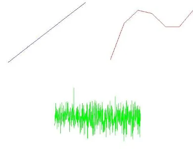
Figure 2: Examples of deterministic and stochastic model. Linear shift (blue), three order polynomio (red), white-noise (green).
3.4 Stochastic model
The stochastic model will be determined after the analysis of the residuals generated when fitting the previous non-continuous function to error measurements. It is expected that these residuals behave as a white noise or Gauss-Markov stochastic process.
4. CONCEPT VALIDATION
4.1 Data set description
controlled area of Dortmund (Germany). The surveyed area was an urban and GNSS challenging scenario, with variable and de-graded GNSS conditions. However, it was an excellent dataset from the imaging sensors point of view with many structured buildings and large variety of features.
The mobile mapping system was an Optech Lynx system, from TopScan GmbH, that includes two laser scanner and two cam-eras. The cameras were mounted looking to each side of a street. The system was mounted on a van and it was driven over a con-trolled area during three hours, resulting in 11 overlapping strips. The interest areas were additionally surveyed to provide a dense network of ground control points. After the survey, the system trajectory was computed using a tightly coupled approach com-bining differential GNSS, IMU and odometer measurements.
The areas used for testing the approach are shown in Figure 3. Two different sections or blocks, marked with blue and orange ellipses, were identified. Each block configuration was selected to represent different situations/configurations that can occur in urban environments with TMM platforms. In an urban environ-ment, a TMM vehicle can survey an interest area several times with the same vehicle driving direction (orange case) or it can survey an area in opposite driving directions, and thus, exploiting and taking benefit from geometric diversity (blue).
Figure 3: Dortmund test areas
Table 1 provides the main characteristics for each of the sections, in terms of used equipment, number of strips, ground control sup-port and number of tie points. Images from four different strips have been used to generate the reference trajectory for the blue section. The vehicle surveyed the area in the same direction three times and a last one in an opposite direction. The surveyed street in the orange block is a one way street, thus, camera images where acquired two times in the same driving direction.
The test areas had a dense network of ground control points and their distribution also varied between sections. For the blue sec-tion, 13 points provided ground control, 7 of them place in the left side of the street. Regarding the orange block, 8 ground con-trol points were used, 5 placed on the right side of the street and 3 of them on the left side. The number of GNSS satellites changed considerably within and between overlapping strips. The number of satellites ranged from one to seven for the blue section, with
TMM equipment
Positioning system Applanix POS LV420
Imaging sensors Optech Lynx cameras
Image size 5.684 x 4.326 mm
Pixel size 3.5µm
No. of ground control points (GCPs) 13
No. of tie points (TPs) 55419
Horizontal Overlap≈ 60
TMM orange area
No. of strips 2
No. of images 121
No. of ground control points (GCPs) 8
No. of tie points (TPs) 22485
Horizontal Overlap≈ 60
Table 1: Dortmund block geometric configuration.
70% of the epochs with equal or less than 3 satellites (Figure 4). The GNSS geometry for the orange section was a bit worse than the blue one with all epochs with three or less satellites. Note that in Figure 4, the tracked satellites for a blue strip with eleva-tion angles higher than 15 degrees are shown in blue, cyan and green. The remaining colours show visible satellites below 15 degrees and not recommended to be used for position estimation. In addition, several GNSS satellites came in or out within few epochs in the same strip.
The reference trajectory was estimated processing the collected information with the Agisoft Photoscan software (Agisoft, 2015). From both camera images, a dense set of points was extracted to be used as non-semantic feature in the adjustment. We benefited from both cameras to work with a stronger geometry. In order to improve the adjustment the system trajectory was also used as observation.
The geometric calibration values, as well as the lever arm and boresight between the cameras, and the IMU, were previously estimated with Agisoft Photoscan using a good GNSS conditions data set. The estimated geometric calibration values are the fo-cal length, principal point, radial and tangential distortion coeffi-cients. That subset included several strips in different directions to help to decorrelate internal camera parameters from the system calibration and from the exterior orientation parameters.
In-house software was developed for estimating trajectory error components, this is, to compare system and reference trajectories.
4.2 Experimental results
Figure 4: Example of tracked GPS L1 satellites for one strip of the blue section.
constellation. It is important to note here that this bias is smaller between the third and the fourth street because of their time dif-ference (less than 5 minutes). Between the first and the second strip there is a difference of 38 minutes, and between the second and the third it is of 12 minutes. Besides the bias, short drift pe-riods broken by several peaks in the trajectory error can also be identified. These peaks are mainly caused by discontinuities in the number of visible GNSS satellites. Moreover, the entrance of a GNSS satellite can produce several epochs of instability during platform trajectory estimation. This effect can be clearly identi-fied in the magenta strip where two big peaks are present.
The error of the heading component of the blue section is shown in Figure 6, following the strip colour scheme of Figure 5. In con-trast to the position error, a significant bias between strips cannot be observed. This is because platform attitude estimation step relies mainly on IMU observations. However, a new GNSS posi-tion after several epochs of inertial-based trajectory might intro-duce also changes in the attitude. This might explain the relevant peak that can observed in the magenta part of Figure 6.
Figure 5: Error component for the y axis from the four overlap-ping strips of blue section.
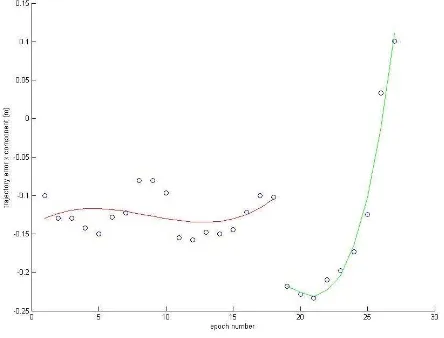
The analysis of the error lead us to model it as a discontinuous third order polynomial. The discontinuities within this function were defined regarding change on strips and also changes in the number of available satellites in each section within a strip. On the other hand, we compute a single stochastic component for each component per strip. Figures 7 and 8 show errors in track axis marked with blue dots for one strip of the blue and one of the orange block. The figures also show the different segments of the error function. In the examples, the deterministic compo-nent was split, within a single strip, in three different segments (red, green, cyan) for the blue section and two (red and green) for
Figure 6: Heading error component from the four overlapping strips of blue section.
the orange section. The comparison of both figures reveals that, at least for the selected sections, the error behaviour is similar, with short drift periods and several discontinuities. The plots for the remaining components are not shown because their similarity with the presented one.
Figure 7: Trajectory error and deterministic part decomposition for the track-axis component of a strip of the blue section.
Figure 8: Trajectory error and deterministic part decomposition for the track-axis component of a strip of the orange section.
stochas-Test Strip Number of Standard deviation position (cm) Standard deviation attitude (mdeg)
deterministic segments x y z he pitch roll
Blue 1 2 2.07 3.63 1.07 43.2 27.2 43.6
2 3 1.17 2.52 0.94 23.9 22.6 37.8
3 3 1.76 3.10 1.02 28.6 23.6 37.8
4 3 5.42 4.45 1.87 59.0 29.0 30.7
Orange 1 2 1.77 2.10 0.93 15.7 21.3 45.0
2 2 2.21 1.98 0.83 17.9 23.2 49.6
Table 2: Stochastic component characterization
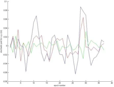
tic model was determined. Figures 9 and 10 show the residuals for each of the error components, corresponding to a single strip for both blue and orange section. The stochastic component of along-track axis component is shown in red, cross-track in blue while height is shown in green.
In Table 2 the number of selected continuous segments for each test are presented together with the standard deviation values of the stochastic part, for each strip and each component. The fig-ures reveal the presence of a stochastic component that can be modeled, in a first approximation, as a white noise process. It can be observed that the stochastic component is lower for the height than for the planimetric components. This can be explained by the use of non-holonomic constraints to reduce the height vari-ation during the initial platform trajectory estimvari-ation. In addi-tion, it can observed that stochastic component is similar in terms of standard deviation for the two sections. As it was expected, the stochastic component is independent of the street or area ori-entation. Beside the comparison between streets, the magnitude of stochastic component, both for position and attitude, remains similar within strips of the same section. The results presented in Table 2 indicate the driving direction has not a significant impact.
Figure 9: Stochastic components of a single strip of blue section.
5. CONCLUSIONS AND FURTHER RESEARCH
We present a strategy to determine as accurately as possible the trajectory error of a TMM system in urban scenarios. The rigor-ous analysis of these reference trajectory against the TMM esti-mated trajectories allows us to characterize the errors of a TMM system for a wide range of environments, and allows exploring in a near term, new and innovative methods for improving TMM trajectory.
The reference trajectory is obtained using extracted non-semantic features from a sequence of images and from a full set of ground control points. The trajectory error is modelled using hybrid
Figure 10: Stochastic components of a single strip of orange sec-tion.
models, that is, combining deterministic and stochastic compo-nents. The deterministic component can be modelled as a non-continuous function composed by linear shifts, drifts or polyno-mial functions. In addition, we introduce a stochastic error com-ponent for modelling residual noise of the trajectory error func-tion.
The proposed approach has been evaluated using real data. The data came from a mobile mapping campaign over an urban and controlled area of Dortmund (Germany), with harmful GNSS con-ditions. The results show the suitability to decompose trajectory error with non-continuous deterministic and stochastic compo-nents.
The work presented in this paper sets the basis for exploring new methods to improve the trajectory of TMM in urban envi-ronments. Further research will be done to explore alternative methods aiming to improve trajectory in urban scenario indepen-dently of the density and type of non-semantic features and/or to reduce the number of required ground control points. In addition, we will explore the use vehicle dynamic constraints for trajectory estimation. Last but not least, we will study the feasibility to ap-ply the same ideas to other mobile mapping platforms that might incorporate consumer-grade sensors.
ACKNOWLEDGEMENTS
The authors thank TopScan GmbH (Germany) for providing the Dortmund dataset.
REFERENCES
Angelats, E. and Colomina, I., 2014. One step mobile mapping laser and camera data orientation and calibration. In: Interna-tional Archives of Photogrammetry, Remote Sensing and Spa-tial Information Sciences, Vol. XL-3/W1, Castelldefels, Spain, pp. 15–20.
Angelats, E., Molina, P., Par´es, M. E. and Colomina, I., 2014. A parallax based robust image matching for improving multisensor navigation in gnss-denied environments. In: Procceding of the ION GNSS+ 2014, Tampa, USA, pp. 2132 – 2138.
Chan, T. O., Lichti, D. and Glennie, C. L., 2013. Multi-feature based boresight self-calibration of a terrestrial mobile mapping system. ISPRS Journal of Photogrammetry & Remote Sensing 82, pp. 112–124.
Elseberg, J., Borrmann, D. and N¨uchter, A., 2013. Algorithmic solutions for computing precise maximum likelihood 3D point clouds from mobile laser scanning platforms. Journal of Remote Sensing 5(11), pp. 5871–5906.
Fern´andez, A., 2012. Final report - ATENEA (Ad-vanced techniques for navigation receivers and applications. http://cordis.europa.eu/publication/rcn/13420en. (Accessed: 24th November 2015).
Gressin, A., Cannelle, B., Mallet, C. and Papelard, J., 2012. Trajectory-based registration of 3D lidar point clouds acquired with a mobile mapping system. In: International Archives of Photogrammetry, Remote Sensing and Spatial Information Sci-ences, Vol. 1-3, Melbourne, Australia, pp. 117–122.
Kersting, A., Habib, A. and Rau, J., 2012. New method for the calibration of multi-camera mobile mapping systems. In: Interna-tional Archives of Photogrammetry, Remote Sensing and Spatial Information Sciences, Melbourne, Australia.
Kutterer, H., 2010. Mobile mapping. In: Vosselman and G. and Maas, (Eds.), Airborne and Terrestrial Laser Scanning, first ed. Whittles Publishing, Dunbeath, Scotland, UK, pp. 293–311.
Leutenegger, S., Furgale, P., Rabaud, V., Chli, M., Konolige, K. and Siegwart, R., 2013. Keyframe-based visual-inertial SLAM using nonlinear optimization. In: Proceedings of Robotics: Sci-ence and Systems.
Nister, D., 2013. An efficient solution to the five-point relative pose problem. In: Proceedings of CVPR03.
Scaramuzza, D., 2011. 1-point-ransac structure from motion for vehicle-mounted cameras by exploiting non-holonomic con-straints. International Journal of Computer Vision 95(1), pp. 74– 85.
Scaramuzza, D. and Fraundorfer, F., 2011. visual odometry [tuto-rial]. IEEE Robotics and Automation Magazine 18(4), pp. 80–92.
Schaer, P. and Vallet, J., 2016. Trajectory adjustment of mobile laser scan data in gps denied environments. In: International Archives of Photogrammetry, Remote Sensing and Spatial Infor-mation Sciences, Vol. XL-3/W4, pp. 61–64.
Skaloud, J. and Lichti, D., 2006. Rigorous approach to bore-sight self-calibration in airborne laser scanning. ISPRS Journal of Photogrammetry & Remote Sensing 61(1), pp. 47–59.
Taylor, C., Veth, M. J., Raquet, J. F. and Miller, M. M., 2011. Comparison of two image and inertial sensor fusion techniques for navigation in unmapped environments. IEEE Transactions on Aerospace and Electronic Systems 47(2), pp. 946–958.
Veth, M. J., 2011. Navigation using images, a survey of tech-niques. Journal of Navigation 58(2), pp. 127–140.