Fundamental equations for growth in uniform stands of vegetation
J.L. Monteith
∗Institute of Terrestrial Ecology, Bush Estate, Penicuik, Midlothian EH26 0QB, UK
Abstract
Applications of the ‘expolinear’ equation for crop growth described by Goudriaan and Monteith [Goudriaan, J., Monteith, J.L., 1990. Ann. Bot. 66, 695–701] are restricted by the assumption that absolute and specific growth rates are both constant in time. To overcome this constraint, a second-order differential equation is derived that may either be integrated to yield the expolinear equation or used with a daily time-step to simulate growth when absolute and specific growth rates are time-dependent. The expolinear equation fitted the biomass of individual organs in a sorghum trial and related quantities such as leaf area per unit biomass. It predicts that an increase in the variability of weather during early stages of growth will usually reduce biomass production. © 2000 Elsevier Science B.V. All rights reserved.
Keywords:Fundamental growth equations; Vegetation; Uniform stands
1. Introduction
Many attempts have been made to derive empirical functions for the increase in biomass (W) with time (t) when plants are grown either in isolation or in stands (Thornley and Johnson, 1990). Commonly, these functions incorporate a specific (or relative) growth rateRdefined as (dW/dt)/Wand introduced by Black-man (1919) as the biological equivalent of a financial interest rate. For seedlings able to grow without com-petition between neighbours,Rusually remains effec-tively constant at a maximum valueRmbecause dW/dt
is proportional to the biomass of organs responsible for resource capture which, in turn, is proportional to total biomass. However, R may decline slowly dur-ing early growth if there is competition for resources between adjacent organs on the same plant. During the main growth period of an arable crop,Rdeclines steadily because of competition between neighbouring
∗Tel.:+44-131-445-4343; fax:+44-131-445-3943.
plants so that, eventually, theabsoluterate of growth
C=dW/dtbecomes almost independent ofW. By assuming that the rate of biomass production per unit of intercepted radiation was constant throughout the whole growing season, that irradiance was also constant, and that leaf area was proportional to to-tal biomass, Goudriaan and Monteith (1990) derived an equation for the time-dependence of crop biomass as a function of Rm and of the maximum absolute
growth rateCmcommonly observed when there is
lit-tle change in the availability of resources from week to week. The equation has the form
W (t )=
C m Rm ln
1+
f
0
1−f0
exp(Rmt )
(1)
where f0 is the fraction of incident radiation inter-cepted by a crop canopy at timet=0. Eq. (1) is ap-propriately described as ‘expolinear’ because biomass increases exponentially with time whentis small and linearly with time when it is large.
As there are few outdoor environments in which it is legitimate to treat Cm and Rm as independent of 0168-1923/00/$ – see front matter © 2000 Elsevier Science B.V. All rights reserved.
time over a whole growing season, Eq. (1) is more useful for demonstrating principles than for predict-ing growth in a specified environment or for analyspredict-ing field measurements. As shown in the following analy-sis, however, bothCmandRmmay be treated as being
time-dependent when Eq. (1) is replaced by a finite difference equation readily handled within a computer program.
2. Derivation of a general expolinear equation
For the short period in which the specific growth rateof a stand may be treated as constant when the environment is constant, theabsolute growth ratemay be expressed as
C= dW
dt =RmW (2)
Integration with respect to time yields the familiar ex-pression for the exponential increase in biomass with time, viz.
W =W (0)exp(Rmt ) (3)
where W=W(0) when t=0. Alternatively, Eq. (2) may be differentiated to obtain the initial ‘growth acceleration’ as
dC
dt =RmC (4)
Eventually, competition between neighbours limits the absolute growth rate toCm, values of which are set by
the availability of resources (water, light, nutrients) per unit land area rather than by physiological demand. To satisfy the final condition that dC/dt=0 along with the initial condition set by Eq. (4), growth acceleration may be expressed as
which is a second-order differential equation in biomass W with C=C0 when t=0. The index n is
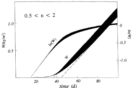
introduced to broaden the applicability of Eq. (5) and its impact is demonstrated in Fig. 1 where W, ob-tained by numerical integration of Eq. (5), is plotted as a function of time when Cm=20 g m−2 per day,
C0/Cm=0.003 andnranges from 0.5 to 2. The initial
Fig. 1. Increase in biomass Wand ln(W) derived from Eq. (7) withRm=0.2 per day,Cm=20 g m−2per day,C0/Cm=0.003 andn ranging from 2 (lowest limits ofWand ln(W)) to 0.5 (uppermost limits).
specific growth rate is almost independent of n and the main impact of n on W is through the intercept on the time axis of the linear portion of the relation betweenW(t) andt. This is the time that is ‘lost’ for resource capture, and therefore, for growth during establishment of the stand. The absolute growth rate approachesCmabout 40 days after emergence (DAE) whenn=0.5 and after about 60 days whenn=2, con-sistent with the fact that many arable crops achieve almost complete ground cover in the second month after emergence.
Eq. (5) derived without reference to a specific pro-cess of resource capture can be integrated twice with respect to time to yield an expolinear function similar to Eq. (1). For the special casen=1, the first integra-tion yields non-dimensional scale of absolute growth rate effec-tively equal toC0/Cm when this ratio is very small as
in most systems of production.
closely resembling Eq. (1) but with the exact limit of W(t)=W(0) when t=0. Commonly,W(0) is much smaller thanW(t) for most of the growing season;Q
may be neglected in the term (1+Q); and when t is
where ‘lost’ time (intercept on the time axis of the linear part of a biomass versus time plot) is given by
tl= −
ln(Q) Rm
(8b)
As Eq. (8a) (the double integral of Eq. (5) whenn=1) has the same form as Eq. (1) obtained by assuming that the distribution of foliage is random, the param-eter n (Eq. (5)) may be regarded as an empirical in-dex of randomness, larger than unity for overdispersed (regularly spaced communities) and smaller for under-dispersed (clumped) communities.
3. Interpretation and extension
By differentiating Eq. (7) with respect to time, it can be shown that
(9) into a similar and more familiar equation for the re-lation between growth rate and light interception,Rm
is replaced byC0/W(0), leaf area indexLis assumed to
be proportional to biomassW, and a time-independent coefficient for light extinction, K, is defined by as-suming thatKL0=C0/Cmwhent=0. The exponential
term in Eq. (9) then reduces to exp(−KL) which is the fraction of lighttransmittedby a leaf area index of L. Neglecting the small fraction of light reflected by a canopy, the term in square brackets is therefore equivalent to the fraction of absorbedradiation that Goudriaan and Monteith (1990) assumed to be pro-portional to growth rate in order to obtain Eq. (1).
Eqs. (4) and (5) were derived by assuming that the growth of plants in a stand is limited initially by plant size, and therefore, by biomass, but eventually be-comes limited by the availability of resources in the
environment. A similar distinction can be made be-tween the relatively slowinitialgrowth of a specific organ (leaf, stem, root) which is likely to depend on its biomass (or ‘sink strength’), and a maximumfinal
rate of growth limited by the availability of assimi-late (or ‘source strength’). The equations may there-fore have limited validity for organs as well as more general validity for plant stands.
If other attributes of growth such as leaf area were to be expolinear functions of time, it would be possible to establish compound quantities such as specific leaf area or leaf area per unit total biomass by dividing one expolinear equation by another. Such quantities will be time-dependent unless values ofRmandC0/Cmare
identical for both processes (see below) so that ‘lost’ times are also identical.
4. Non-dimensional expolinear equation
To compare the growth of different species in the same environment or of different organs on plants within the same stand, it is convenient to write Eq. (8a) in the non-dimensional form
W∗(t )=ln{1+exp(t∗)} (10) whereW∗(t)={W(t)−W(0)}(Rm/Cm) is a non-
dimen-sional mass andt∗=Rm(t−tl) a non-dimensional time.
As measurements of biomass in a stand are commonly deferred until W∗(t) is much larger than W∗(0), the latter term can usually be neglected.
During the initial stages of growth when exp(t∗) is much less than 1, Eq. (8a) assumes a lower limit of W∗=exp(t∗), implying that biomass increases ex-ponentially with time. If t∗ increases until exp(t∗)
is much larger than 1, the equation has an upper limit W∗=t∗ so that biomass increases linearly with
time.
5. Field tests in a quasi-constant environment
Fig. 2. Increase in total biomass of sorghum grown during rainless weather at ICRISAT, Hyderabad, India. (h) No irrigation or applied N; (s) no irrigation and 150 kg N/ha; (d) irrigation and 150 kg N/ha.
dry season in the semi-arid tropics, crops grow on stored water during a rainless period when the sky is usually cloudless so that radiation is uniform and mean temperature declines only slowly with time. Observations on the growth of sorghum in such an environment have been reported by Rego et al. (1998) and by Singh et al. (1998) working at the International Crops Research Institute for the Semi-Arid Trop-ics (ICRISAT), Hyderabad. They grew a sorghum cultivar (SPH-260) on a deep Vertisol at six levels of fertilization (0–150 kg N/ha) and at two levels of irrigation (zero after initial wetting throughout the profile and restoration of the profile to field capacity approximately every 2 weeks from emergence until 50 days later). Three replicate samples were obtained from all treatments, weekly for leaves and stems and every 2 weeks for roots.
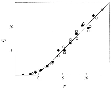
In Fig. 2, total biomass is plotted as a function of time for three contrasting treatments. Expolinear equa-tions (parameters in the legend of Fig. 3) fit the data well and illustrate an important feature:Cm doubled in response to the application of water and nitrogen. In contrast,Rm andC0/Cmwere effectively independent of treatment, implying thattl(Eq. (8b)) was also inde-pendent of treatment. Therefore, measurements for all treatments fall on the universal growth curve obtained by plotting the normalized biomassWRm/Cm against
normalized timeRm(t−t1) (Fig. 3).
In this trial, the biomass of individual organs also increased with time in an expolinear fashion. How-ever, the growth of leaves (Fig. 4) stopped abruptly at aboutt∗=8 corresponding to 60 DAE when anthesis was recorded. In contrast, stems and roots continued to grow until physiological maturity at aboutt∗=17
corresponding to 90–95 DAE.
Fig. 3. Non-dimensional plot of total biomass (W∗=WRm/Cm) for
sorghum as a function of non-dimensional time from emergence (t∗=Rm[t−tl]) obtained from the data in Fig. 2 assuming identical
Fig. 4. Non-dimensional plot of biomass for leaves of sorghum grown at six rates of nitrogen (0, 30, 60, 90, 120, 150 kg/ha) ranked by size of the symbol.
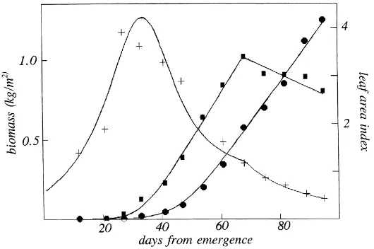
The expolinear increase in biomass with time was accompanied by an expolinear increase in leaf area un-til anthesis. Thereafter, leaf area decreased with time at an approximately constant rate. Fig. 5 illustrates this behaviour for a treatment (150 kg N/ha with irrigation) in which the ‘lost’ time for leaf area was 32 DAE com-pared to 45 days for total biomass. In consequence, the leaf area per unit biomass increased rapidly until about 30 DAE and then decreased equally rapidly un-til maturity at about 100 DAE. The curve representing leaf area index per unit biomass was obtained in three
Fig. 5. Leaf biomass (d), leaf area (j) and leaf area ratio (+) for sorghum (see text).
stages: (a) fitting leaf area to an expolinear equation up to 60 DAE and to a linear equation for the sub-sequent senescent phase; (b) fitting total biomass to a second expolinear equation; (c) dividing the output from (a) by the output from (b). A general inference from this analysis is that relatively small differences in lost time for two components of growth can be re-sponsible for a more complex response to time in the ratio of these components. Interpretation of growth in such terms has potential for revealing substantially more information about underlying processes than the traditional fitting of arbitrary empirical functions.
At least in a quasi-constant environment, it appears that the expolinear equation may be applicable to the growth of individual organs as well as to ontogenetic changes of compound quantities such as leaf biomass or nitrogen content per unit leaf area. The procedure to be followed in a variable environment is discussed in Section 6.
6. Yield and weather variability
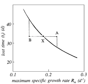
Fig. 6. Dependence of lost time tl on specific growth rate Rm whenC0/Cm=0.004.
dependence has not been explicit, but the dependence of ‘lost’ time on the maximum specific growth rate
Rm may be a significant factor.
Laboratory evidence suggests that Rm may be
as-sumed to increase linearly with temperature at least over a narrow range. As dtl/dRm is negative but d2tl/dRm2 is positive (Fig. 6), any increase inRm(e.g. from X to A) as a result of an increase in temper-ature, say, will be responsible for a decrease in tl
smaller than the complementary increaseintl (from
X to B) induced by a negative temperature fluctua-tion of identical magnitude. It follows that, during the establishment of a stand when growth is strongly dependent on the magnitude ofRm, fluctuations in an
environmental factor such as air temperature causing
Rm to fluctuate will result in a loss of production,
albeit small in many circumstances. In the main pe-riod of growth, however, where the growth rate is dominated by the value of Cm, production (at a rate
proportional to Cm) should not be affected by small fluctuations in the growth rate about its mean value.
Eq. (4) has the important property that it defines the relation between d2W/dt2and dW/dtin terms of initial relative and final absolute growth rates but not in terms of the initial biomass or the initial absolute growth rate. It is therefore possible to use the equation to obtain the increase in growth rate and biomass with time numerically, adopting, for example, a daily time-step and values ofRm andCm that depend on the state of
the environment, and therefore, on time. If the time
step isδt, the crop growth rateC(t) (=dW/dt) on Day
tis given by
C(t+δt )=C(t )+δtdC(t )/dt (11)
where, from Eq. (5) (neglecting the small termC0),
dC(t )
dt =C(t )Rm(t )
1− C(t )
Cm(t )
(12)
Biomass at the start of Dayt+1 is then evaluated as
W (t )=W (t−δt )+δt C(t ) (13)
This behaviour is illustrated in Fig. 7 where the cir-cles represent biomass estimated as a function of time using Eq. (7) withconstantvalues ofRm(0.2 per day)
and ofCm (10 g m−2 per day for C3 species — open
circles; and 20 g m−2 per day for C4 species — full
circles). The two shaded portions were obtained with the same values ofCm but with environmental fluc-tuations introduced by assigning random daily values between 0.18 and 0.22 per day toRm. In practice,
fluc-tuations of this order could be a consequence of daily mean temperature fluctuating by±2◦C about a mean
of 20◦C, assuming that the relative growth rate is
pro-portional to temperature over the range considered.
7. Conclusions
The differential equation (Eq. (5)) that forms the basis of the expolinear equation (Eq. (7)) provides a new method for simulating the growth of crop stands and possibly of their components. Unlike more com-plex systems of simulation, it is based on a secure foundation of calculus and operates with a minimum of parameters and arbitrary constants. The main prob-lem in using the equation practically is common to all types of modelling which assume values for the dependence of dominant parameters (Cm, Rm andQ
in this paper) on physiology, management, and the state of the environment both above and below the ground.
References
Blackman, V.H., 1919. The compound interest law of plant growth. Ann. Bot. 30, 353–360.
Goudriaan, J., Monteith, J.L., 1990. A mathematical function for crop growth. Ann. Bot. 66, 695–701.
Rego, T.J., Monteith, J.L., Singh, P., Lee, K.K., Nageswara Rao, V., Srirama, Y.V., 1998. Response to fertiliser nitrogen and water of post-rainy season sorghum on a Vertisol. 1. Biomass and light interception. J. Agric. Sci. 131, 417–428.
Semenov, M.A., Porter, J.R., 1995. Climatic variability and the modelling of crop yields. Agric. For. Meteorol. 73, 265–283. Singh, P., Monteith, J.L., Lee, K.K., Rego, T.J., Wani, S.P., 1998.
Response to fertiliser nitrogen and water of post-rainy season sorghum on a Vertisol. 2. Biomass and water extraction. J. Agric. Sci. 131, 429–438.