SATELLITE-BASED RADAR MEASUREMENTS FOR VALIDATION OF
HIGH-RESOLUTION SEA STATE FORECAST MODELS IN THE
GERMAN BIGHT
A. Pleskachevsky a,* , C. Gebhardt a, W. Rosenthal a, S. Lehner a , P. Hoffmann b , J. Kieser b , T. Bruns b , A. Lindenthal c , F. Jansen c , A. Behrens d a
German Aerospace Center (DLR), Remote Sensing Technology Institute, Maritime Security Lab, Henrich-Focke-Straße 4, 28199 Bremen, Germany – [email protected], [email protected],
[email protected], [email protected] b
German Meteorological Service (DWD),
Bernhard-Nocht-Str. 76, 20359 Hamburg, Germany - [email protected], [email protected], [email protected] c
German Maritime and Hydrographic Agency (BSH),
Bernhard-Nocht-Str. 78, 20359 Hamburg, Germany - [email protected], [email protected] d
Helmholtz Center Geesthacht (HZG), Institute of Coastal Research, Otto-Hahn str.1, 21502 Geesthacht, Germany – [email protected]
Commission VI, WG VI/4
KEY WORDS: Ocean waves, coastal processes, wave modeling, high resolution, remote sensing, radar satellites
ABSTRACT:
Remote sensing Synthetic Aperture Radar (SAR) data from TerraSAR-X and Tandem-X (TS-X and TD-X) satellites have been used for validation and verification of newly developed coastal forecast models in the German Bight of the North Sea. The empirical XWAVE algorithm for estimation of significant wave height has been adopted for coastal application and implemented for NRT services. All available TS-X images in the German Bight collocated with buoy measurements (6 buoys) since 2013 were processed and analysed (total of 46 scenes/passages with 184 StripMap images). Sea state estimated from series of TS-X images cover strips with length of ~200km and width of 30km over the German Bight from East-Frisian Islands to the Danish coast. The comparisons with results of wave prediction model show a number of local variations due to variety in bathymetry and wind fronts.
1. INTRODUCTION
1.1 Novel satellite borne SAR for oceanography
The estimation of marine and meteorological parameters is an important task for operational oceanographic services. In comparison to in-situ buoy measurements at a single location, remote sensing allows to cover large areas and to estimate the spatial distribution of investigated characteristics. The spatial validation of forecast data, e.g. sea state and surface wind, through remote sensing data can visibly improve the forecast quality and help explain natural phenomena beyond ordinary circumstances like storm front propagation, gusts and emergence of wave group with extreme wave height (Lehner et al., 2012, 2013, Pleskachevsky et al., 2012).
Space borne SAR (Synthetic Aperture Radar) as a remote sensing instrument is a unique sensor which can cover large areas and provide two dimensional information of the ocean surface. Due to its high resolution, daylight and weather independence and global coverage, space borne SAR sensors of the latest generation are particularly suitable for ocean and coastal applications. Over the last years, a number of new high resolution X-band radar satellites have been launched, which provides the possibility to image and measure the sea surface with high resolution e.g. TerraSAR-X (TS-X), TanDEM-X(TD-X) and COSMO-Skymed satellites. This opens a new perspective for investigating sea state and connected processes in coastal areas, where spatial variability in sea surface play an important role. A wide spectrum of features and signatures of sea state and derived parameters are simultaneously involved and can be observed in high resolution images including surface wind and gusts, individual waves and their refraction, wave braking effects, etc. Knowledge of basic geophysical processes and its imaging mechanism is necessary for successful processing of images and for organization of NRT services to
provide the information to interested users like the German Meteorological Service (Deutscher Wetterdienst, DWD).
1.2 Objectives: improving of sea state prediction in German Bight and intertidal zones of North Sea
The German Bight in the North Sea is characterized by a strong dependence on tides in complex topography with number of islands and shoals. Fast-changing of water levels and local currents reaches more than 2m·s-1 as well as emergence of numerous sandbars and shoals greatly influences the wave propagation.
The scientific and technical tasks presented in this paper were on the one hand the improvement of forecast services especially in coastal areas by development of high resolution coastal model (1). On the other hand, new algorithms were to be developed for estimation of meteo-marine parameters from SAR images in coastal waters with high accuracy (2) and likewise products were to be conceived for NRT services (3). As a result an automatic chain “Coastal waves prediction/NRT SAR acquisition and processing/delivery on DWD and validation” was developed.
the fact that disembarking height from a boat onto an offshore construction (e.g. wind farm) may not exceed 1.2m. In case HS
exceeds 1.2m, the disembarking is too hazardous for crew members and the transport ship must return back to the harbour. Such works are planned in advance and inaccurate predictions cause high additional costs.
1.3 Coastal processes and forecast services
The wave models of the third generation have been developed and used for sea state prediction, e.g. WAVEWATCH III used by NOAA (http://polar.ncep.noaa.gov/waves/) and UKMET (United Kingdom Meteorological Office), and WAM model used by forecast services in Europe like ECMWF (European coastal areas: wind input implies well-timed atmospheric front propagation and interaction in shallow water caused between waves, currents and the sea bottom becomes important. Currents and the sea bottom cause waves to refract, get dampened, become steeper and break. The wave energy dissipates and transfers into turbulence and acceleration of flow currents (radiation stress).
The high resolution Coastal Wave Model (CWAM) for the German Bight and the western Baltic Sea has been developed by DWD and BSH in cooperation with the Helmholtz-Zentrum Geesthacht (HZG). CWAM is based on the Wave Model
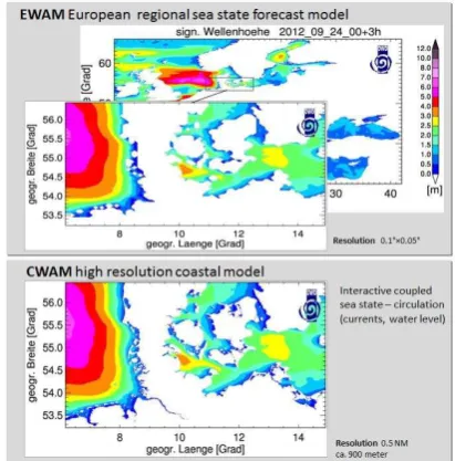
Figure 1. Conventional EWAM sea state forecast and new high
resolution coastal model CWAM (0.5NM=~900m). Local differences of resulting HS in coastal areas are in the range of
meters because of more structures in bathymetry (1) and rapid change of water level and circulation currents by tides not resolved by EWAM in intertidal Watt zone (2).
A product combines forecasts and a near real time assessment with high-resolution satellite data. Local differences of resulting
HS EWAM/CWAM in coastal areas are in the range of meters
because of more structure in bathymetry (1) and rapid change of water level and circulation currents by tides (2) (see Fig.1).
2. REMOTE SENSING NEW TECNIQUE
2.1 Satellite borne SAR data for oceanographic applications
In this paper the data from TerraSAR-X (TS-X) and its twin TanDEM-X (TD-X) were used for validation. The X-band SAR satellite TS-X (launched in 2007) and its twin TD-X (launched in 2009) operates from 514km height at sun-synchronous orbit with ground speed of 7km·s-1 (15orbits per day). It operates with a wavelength of 31mm and a frequency of 9.6GHz. The repeat-cycle is 11 days, but the same region can be imaged by different incidence angles after three days dependent on scene latitude. Typical TS-X incidence angles range between 20° and 55°.
TS-X operates five different basic imaging modes with different spatial resolution: from High-Resolution Spotlight 5km×10km to about 280km×400km wide ScanSAR mode with 40m therefore not suitable for coastal applications.
Methods to derive wind speed and sea state using simple empirical models from high-resolution SAR data have been developed by DLR: a new nonlinear wind algorithm XMOD-2
(Li and Lehner, 2013) and a new empirical model function XWAVE-2 (Lehner et al., 2013) for obtaining significant wave height from X-band data. Both algorithms are capable of taking into account fine-scale effects in coastal areas. As the sea state is directly connected to local wind, the wind information form the same SAR image will be taken for filtering of noise and checking of sea state. For coastal areas, the sea state algorithm was adapted and tuned again to account for non-standard coastal effects.
2.2 Surface wind from TerraSAR-X data
The SAR wind field retrieval approach was first developed for C-band SAR provided by, for example, ERS-2 and ENVISAT ASAR. These approaches utilized an empirically derived Geophysical Model Functions (GMF) that related local wind conditions and sensor geometry to radar cross section values (e.g. CMOD4 or CMOD5). To utilize the new SAR systems, an X-Band linear algorithm XMOD-1 and later a nonlinear XMOD-2 was established for VV and HH polarized data to obtain the wind fields (Li and Lehner, 2013). The relationship between X-band radar cross section and wind speed, wind direction and incidence angle in XMOD-2 is given by:
)) parameters Bi with i=0,1,2 are tuned using the measurement data
produced by airflow turbulent eddies at the boundary. Shadows global atmosphere and surface conditions for 45-years) were used to tune the algorithm. The results were validated using in-situ measurements from collocated buoys and modelled data with different resolution (HIRLAM model and DWD COSMO). The wind field can be retrieved with 20m resolution by the XMOD algorithm for TS-X images. In contrast to the previously developed XMOD-1, XMOD-2 consists of a set of nonlinear GMFs and therefore depicts the difference between upwind and downwind of the sea surface backscatter in X-band SAR imagery. By exploiting 371 collocations with in situ buoy measurements which are used as the tuning dataset together with analysis wind model results, the retrieved TS-X/TD-X sea surface wind speed using XMOD-2 shows a close agreement with buoy measurements with a bias of -0.32m∙s-1, an RMSE of 1.44m∙s-1
and a scatter index (SI) of 16.0%. Further validation using an independent dataset of 52 cases shows a bias of -0.17m∙s-1, an RMSE of 1.48m∙s-1
, and SI of 17.0% comparing with buoy measurements (Li and Lehner, 2013).
2.3 Sea state from TerraSAR-X data
Several retrieval algorithms to derive the two-dimensional ocean wave spectrum or integral wave parameters from SAR information beyond the so-called azimuth cut-off wavelength. For TerraSAR-X images this cut-off is about 30m for range traveling waves, and the non-linear effects like velocity bunching are visibly reduced in comparison with earlier SAR mission due to lower orbit of 500km (e.g. ASAR with 800km orbit).
An empirical XWAVE-1 model for obtaining integrated wave parameters has been developed for X-band. The algorithm is based on analysis of image spectra and uses parameters fitted with collocated buoy data and information on spectral peak direction and incidence angle. The new developed XWAVE-2 algorithm to derive significant wave height directly from TS-X SAR image spectra (no transferring into wave spectra) is
directional wave number Image Spectrum (IS). Parameters c1-c4
are the coefficients tuned to various data sets and dependent on incidence angle θ. They are determined from a linear fitting between EIS and the collocated significant wave height,
computed by the DWD wave model, collocated buoy measurements, WaMoS-II (Wave Monitoring System) and Radar altimeter data (Bruck and Lehner 2013). The integration domain chosen is limited by minimal and maximal wavelength in order to avoid the effects of wind streaks by turbulent boundary layer and the “cut-off” effect of SAR imaging of short
sea surface waves. The values are set to Lmin=30m and
Lmax=600m, which corresponds to kmax=0.2 and kmin=0.01 in
deep water. The TS-X Image Spectrum IS(k) is obtained through the Fast Fourier analysis (FFT) done on a subscene of the radiometrically calibrated TS-X/TD-X intensity image. Generally, the algorithm has been tuned with the NOAA buoys in open ocean where hundreds of TS-X scenes were acquired especially for this purpose with scatter index SI for significant wave height SIHsXWAVE/BUOY=0.21 and SILXWAVE/BUOY=0.13 for wavelength (Lehner et al., 2013).
2.4 Improving of sea state algorithm for coastal areas
The XWAVE algorithm developed for open sea works well for several sub-scenes with well-pronounced waves checked by a homogeneity test. For space-coverage analysis of scenes and automatic NRT services it was necessary to develop and add the series of filters and corrections. A direct implementing of GMF
Eq.2 in coastal area leads to more than 50% errors of processed data with outliers in the range of meter for HS. The sources of
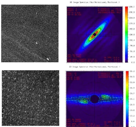
error are in first place artefacts in SAR imagery typical for Wadden/mudflat coastal waters: sand banks, wave breaking, ships, current boundaries and atmospheric fronts and even internal waves structures. All these objects impact the image spectra. Such spectral perturbations result in an integrated value which yields a contribution to total energy that is not connected to sea state (Fig.2).
The core of the newly developed Sea Sate Processor (SSP) for both HH and VV polarisation consists of (see Fig.3):
Step-1: sub-scene pre-filtering (remove image intensity outliers like ships, buoys etc. based on local intensity statistics),
Step-2: calculation of XMOD-2 wind,
Step-3: spectral analysis of subscene (FFT, integration and spectral parameters e.g. noise level),
Step-4: new XWAVE-2 GMF (SSP core),
Step-5: checking of results using wind speed and integrated spectral parameters (e.g. long structures like sand banks produce high spectral values in domain k<0.01 and can be separated).
Figure 2. Examples of artefacts in TerraSAR-X sub-images
Figure 3. Flow chart of Sea Sate Processor (SSP).
The XWAVE algorithm Eq.2 has been repeatedly validated and adapted for coastal sea state in order to improve the existing function. In the first instance the CWAM model data were used for spatial-temporal validation in order to understand the source of outliers and create the additional terms necessary to compensate perturbations. Model data served thus only to establish an appropriate ansatz function, that is capable of representing all spectrally significant phenomena. Although the model reproduces the spatial distribution of sea sate correctly, the model scatter index for buoy positions and TS-X images date is SIHsCWAM/BOUY=0.23 and the values are sometimes overestimated by 0.5-1.0m (total mean value of HS=1.5m for
buoy locations with mean value of 2.5m for storm conditions). In a second step, re-tuning of coefficients of the ansatz function (found in the previous step) in order to fit this function to the buoy measurements have been done.
To compare TS-X data with model results, TS-X scenes were processed with 3km×3km step (~10 sub-scenes for range and ~15 sub-scenes for azimuth directions 10×15=150 sub-scenes per StripMap image with squares of ~5km×5km). In total, 21 data sets were used (TS-X and CWAM model results at the same day, time differences in order of maximal 10min between model output and TS-X acquisition time). The comparison was made for NN/MSL (normal null/mean sea level) depths >5m in order to exclude dry sand banks during ebb and has about 9000 collocated data pair TS-X/CWAM.
After comparison, XWAVE_C (Coastal) functionEq.2 is: 5 5 4 4 3 3 2 2 1
1 _
)
tan( a B aB aB aB E
B a
HsXWAVE C IS (3)
where a1-a5 are coefficients (constants) and B1-B5 are functions
of spectral parameters. B1 represents noise scaling of total
energy EIS (short wind waves and their breaking produce an
additional noise that influences non-linearly resulting energy),
a2B2 term represents wind impact according to the original
XWAVE Eq.2. The terms a3B3 and a4B4 are corrections for
eliminating the impact of short (e.g. wave breaking induced) and long (e.g. wind streaks) structures in the SAR image. These structure results in spectral peaks with modes not directly connected to sea state. a5B5 is a correction for outliers produced
by extra-large structures like sand banks or ship wakes which have not been filtered by Step-1.
During data tuning it became clear that not every TS-X scene shows well-pronounced sea state like swell waves and more than 50% of images cannot be used in the traditional way using Eq.2.However, now using the improved function Eq.3 already a small signal in the SAR-image (no wave-like shaped structures but only speckle), e.g. during calm weather condition ~ 2m∙s-1
< U10< 8m∙s
-1
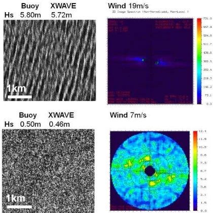
is enough to deduce the sea state that is responsible for noise occurrence in SAR image.More precisely, a large number of wave crests, which are small moving targets, may be not imaged individually by SAR in original shape, but jointly produce radar echo with intensity proportional to their speed and amplitude. Fig.4 demonstrates two examples of different sea state at the same position near buoy “Elbe”. The subscenes were shown near the buoy location. The values of spectral maxima differ by orders of magnitude. The storm acquisition on 09.12.2011 at 05:52 shows well pronounced swell waves. Under lower wind condition on 07.01.2015 at 17:19, wave-like structures are hardly visible. Nerveless HS can
be accurately estimated based on noise properties of spectra and wind information.
2.5 Sea state NRT Services
The Sea Sate Processor (SSP) which includes the XWAVE algorithms was extended and adapted for automated NRT services with 40 input control parameters (FFT size, raster analysis step, ship filtering properties, etc.). The SSP was installed at the Ground Station “Neustrelitz” to provide an operational service and is currently being tested. The delivery of
Figure 4. Two examples of different sea state at the same
position buoy “Elbe”. TerraSAR-X storm acquisition on 09.12.2011 at 05:52: long waves are well pronounced. Low wind condition on 07.01.2015 at 17:19: wave-like strictures are hardly visible, nevertheless, HS can be accurately estimated
NRT products from “Neustrelitz” to the user (e.g. DWD) occurs by E-mail. The attachment includes a text file (.txt) with the data (lon, lat, Hs), the Google Earth file (.kmz) for an illustration of an image file (.jpg).
The program interface allows the user to change the pre-installed properties of automatic data processing and output. The output writing of four text-file types is possible with additional graphic view as TIFF files for processed image, sub-scenes, 2-D and 1-D spectra (optional):
TSX_acquisitiondate_mean-values.txt contains the mean
values of all parameters for the scene (Hs, wind, intensity, incidence angles, geo-coordinates, etc.);
TSX_acquisitiondate_waves.txt contains only Hs with details of the geo-coordinates (for extern users);
TSX_acquisitiondate_results.txt - all parameters such as
integrated energy, noise and other details for each analysed subscene are stored.
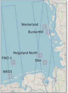
TSX_acquisitiondate_special-points.txt contains infor-mation for minimal distance of subscenes analysed to special points (e.g. buoys and offshore construction) specified in input file spetial-points_input.txt (for the German Bight, 6 spatial points were used: measurement piles, wave rider buoys, see Fig.6).
3. RESULTS
3.1 Data ordering, acquisition and processing
The CWAM model runs at the DWD since 01.01.2013. For validation of XWAVE, a series of images was ordered over the German bight in such a way as to cover the German Bight coastal areas and measurement buoys (see Fig.5): The scenes were ordered twice in series of 3 months for each possible overflight (or each 2/3 day). Additionally, individual images were ordered in order to cover interesting weather conditions in coastal areas and over offshore wind parks (e.g. over FiNO-1 research platform). A series of images ordered by other users were downloaded from the EOWEB (Earth Observation Web) catalogue (e.g. for ship detection, oil detection or wind analysis for wind parks).
When ordered, only 30% of the ordered scenes were actually acquired. This is due to the low priority of the science-user. In 2015, this ratio should improve due to installation of a new receiving antenna at the ground station “Neustrelitz”.
Figure 5. Concept for TerraSAR-X scenes ordering for CWAM
wave model validations: two typical ascending and descending overflights collocated with 6 available buoys in the German Bight in wave model domain. Each acquired scene consists of 3-6 single images.
Figure 6. Uncertainties for comparison of TS-X derived sea
state and buoy: TerraSAR-X Stripmap typical analysis with subscenes (left) and subscene with buoy (right); buoy represents statistics of a sector with sea state propagating to buoy (red marked area) integrated over time (typically 20min time series). TS-X represents “frozen” HS from spatial (snap shot) statistics
of sub-image which includes more spatial variability than buoy data.
As a result, in 2013-2014 a total of 43 TS-X buoy-collocated scenes in the German Bight with 154 images are available and used. In March 2015, this number increased to 46 Scenes with 173 images. However, the data since October 2014 were not anymore included for XWAVE tuning but are only used to verify the statistics.
TS-X scenes were processed with step of 3km×3km (~10×15=~150 subscenes per image). The collocations were done with a time window of +/- 10min for comparison with model data and +/-20min for buoys (slightly varying recording period). CWAM hourly output is at 6:00 and 18:00 UTC and acquisition time for TS-X is 05:50-06:10 for descending orbit and 17:50-18:10 for ascending orbit in German Bight. Spatial collocation occurred in a domain up to 5km (subscene size). A source of uncertainties for comparison lies in the fact that a buoy represents statistics of a small sector of sea state propagating towards the buoy, integrated over time (typically 20min time series). TS-X represents HS from statistics of a
wider “frozen” area (snap shot) which includes more variability than buoy data due to e.g. bathymetry disturbing the homogeneity of sea state. As a result, HSbuoyand HSTSX are the
same only in case no temporal (~20min) and no spatial variations (~5km×5km) occur in sea state statistics (see Fig.6).
3.2 Statistics
Local comparison TS-X/Buoy was conducted for 6 stations in
the German Bight (Fig.5). Actually, a total of 46 TS-X Scenes (events) with 173 Images and 72 buoy collocations (collocation around 20min and up to 5km spatially) were available and analyzed. The scatter index SITSX/BUOY=20% was obtained for all data. Currently the scatter index (the same buoys) for DWD coastal wave model has the same value SICWAM/BUOY=20%. However, the model tends to overestimate HS while TS-X
values are scattered more symmetrically around the buoy values. Fig.7 and Fig.11 show the same comparison of TS-X XWAVE_C/Buoy measurements in the form of a scatter-plot for all data and a bar-plot for 2013-2014.
Statistical analysis shows the averaged value of collocated HS to
be about 1.5m in the German Bight. Acquisition with HS>2.5m
occurred quite rarely. It was only two times possible to acquire a storm with HS>5m (09.12.2011 and 10.12.2014). For this
Figure 7. Total comparison of all available data in German Bight
2013-2015 including a storm on 09.12.2011: 46 TerraSAR-X Scenes (overflights/events/days) with 173 Images and 72 buoy collocations (collocation around 20min and up to 5km spatially). It is interesting to note that according to earlier studies at HZG in the German Bight generally only 0.3% of all cases the Hs
value exceeds 2.5m for local wind U10<12m∙s-1. This statistics is
based on 10-yers sea state reanalysis with the WAM model for the North Sea for 1990-2000 and show a strong dependence of sea state on local wind.
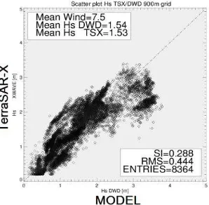
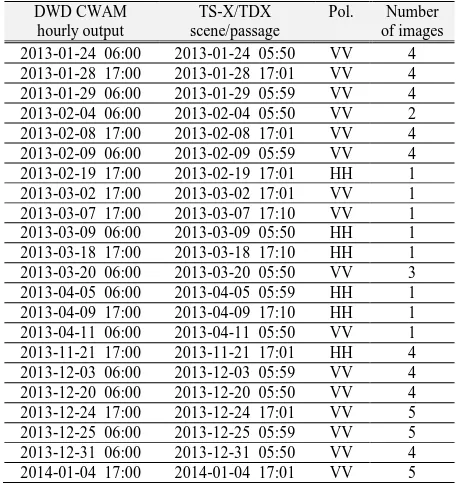
As mentioned above, the spatial comparison TS-X/CWAM
model results was done for 21 collocated CWAM data sets
(days) with 64 TS-X images and 83664 collocated HS pairs
HSTSX/HSCWAM (depths >5m) (Tab.1). The scatterplot is shown
in Fig.8. The scatter index amounts to SITSX/CWAM =0.28 and is higher than SITSX/BUOY=0.20 for comparisons TS-X/Buoys. This value was previously 0.23 by tuning with CWAM results only. However, for this case, the TS-X/Buoy comparison was not satisfactory (inaccuracy of the model includes SICWAM/BUOY =0.23 for buoy locations). Thus the coefficients of XWAVE_C GMF were later adapted in order to shift the ansatz function without changing the generic ansatz function type developed before by using CWAM model data only. In Fig.8, it is clearly visible and individual scenes can be separated as “clusters”. An analysis of surrounding parameters reveals that the overestimation of forecasted HSCWAM is often connected to
overestimated local wind. The atmospheric fronts and gusts (wind input from Atmospheric Model) enter evidently the area with a time delay. The second source of overestimation of sea state in the costal model can be explained by local bathymetry influence. The soft seabed topography in German Bight can change fast due to storms so that model topography can be out of date.
Figure 8. Total comparison of data set Tab.1 TerraSAR-X
/CWAM in German Bight 2013-2014: 21 TerraSAR-X Scenes (events) with 64 images and 8364 collocation pairs (TS-X processing with a raster step of 3kmx3km and for depth>5m MSL).
3.3 Examples
Spatial comparison displays generally correlated sea state spatial distribution (pattern) by TS-X derived data and CWAM model data. The differences are often visible as a local variation of sea state generated by time-shifted wind front (model input hourly) and/or over misplaced sand banks (model bathymetry resolution 900m). Fig.12 presents a spatial validation of a descending TS-X scene consisting of 5 images on 25.12.2013 at 05:59 UTC. The middle sub-figure shows TS-X XWAVE_C values plotted over CWAM model results at 06:00 UTC. The model shows a front with HS>2m (red color) at the Danish
coast, corresponding with wind ~11m∙s-1. TS-X XWAVE_C HS
values are about 1.5m with local wind ~8m∙s-1. With a moving wind front and averaged seas state propagation speed of 10m∙s -1
, it can cross the area covered by the TS-X image (30km streak) in less than an hour. Fig.9 shows an example of wavelength comparison for sequence’s (Fig.12) image-2. Peak wavelengths derived from TS-X image spectra were superimposed on wavelength derived from CWAM model results from peak period and actual local depth. Both, model and TS-X show identical spatial distribution in wavelength domain 60m-100m with local differences in order of 10m-20m.
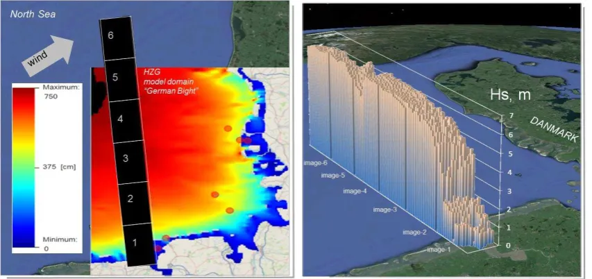
Another example is one successful acquisition of a storm on 10.12.2014 at 17:19 UTC. A sequence of 6 TS-X StripMap images covers the German Bight completely. The wind increases up to 18m∙s-1 (XMOD-2) at the position of Lightship “TWEms” provided by BSH (Meteorology: DWD) located at 54.1666N and 6.3500E reported wind around 17.5m∙s-1. Fig.13
shows model results of wave model of HZG (COSYNA) at 18:00 UTC and 3-D HS derived from TS-X images using
XWAVE_C algorithm. A time delay of 40min does not play a role according to model time series: from 00:00 UTC the wave height increases permanently from 4m to about 7m until 16:00 and remains constant further on until 11.12.2014. It can be clearly seen that TS-X data reproduce the same spatial patterns including wind dependent growth of sea state (fetch). On the other hand, TS-X has more spatial variability as the smoother model data.
Figure 9. An example of comparison for wavelength derived from
4. DISCUSSION
The collected data show that sea state which propagates in azimuth direction (SAR flight) is minimally disturbed by nonlinear effects and results in spectra with practically no visible cut-off while the sea state moving in range direction (to SAR) is strongly perturbed by non-linear artifacts and defocussing. Often these distortions for near-range moving waves are so strong that the waves itself cannot be seen underneath the streak-structures. Such distorted sea state results in spectra with well-visible “cut-off” with a ratio (noise level inside cut-off)/(noise level outside cut-off) in the order of 3-5. These results show that the strongest impact of nonlinear effects (velocity bunching and defocusing) is due to the radial component of phase velocity of the wave (=0 in case of azimuth traveling waves and maximal for range traveling waves =cos(θ)∙wavelength/period) rather than local orbital wave velocities. Contrary to expectations, Fig.10 demonstrates that the more waves are turned towards the SAR range direction, the more distorted and defocused they are by non-linear effects. Additionally, it can be seen that in coastal areas for short waves with wavelength <~50m, a “cut-off” is visible. No azimuth components of traveling waves but only range components can be observed in TS-X SAR images.
Figure 10. Example for three situations of TerraSAR-X
acquisitions for similar sea state traveling in different directions (peak wavelength ~80m-100m): azimuth traveling (left), range traveling (right) and intermediate situation. The azimuth traveling waves are minimally distorted by non-linear effects, the shape of image spectra approaches shape of wave spectra; for 45° traveling waves the distortions are already visible, and for range traveling waves, the distortions dominate.
5. SUMMARY AND OUTLOOK
The algorithms to derive sea state integrated parameters from X-band SAR data were adapted for coastal applications. An NRT version of the Sea State Processor was made operational and processed data were provided for the validation of forecast Wave Model CWAM of German Weather Service in the German Bight in order to improve the predictions in coastal areas and at offshore constructions. It is planned to extend and adapt the algorithms and developed NRT products for Sentinel satellite C-Band SAR data.
ACKNOWLEDGEMENTS
This study was supported by DLR Space Agency with project DeMARINE-2 SEEGANGSMONITOR and by BMVI (German Federal Ministry of Transport and Digital Infrastructure) with project “Development of Sea-State-Monitor to improve Sea State prediction systems” N 97.0304-2012
The authors are grateful to the team of DLR ground station “Neustrelitz” for active cooperation and organization of NRT service-chain for providing data to users.
The authors gratefully acknowledge COSYNA data portal by HZG, NWS (North West Shelf) Portal by BSH and EMODnet
COSYNA data web portal CODM http://codm.hzg.de/codm/
Kieser, J., Bruns., T., Behrens, A., Lehner, S. and A. Pleskachevsky, 2013. First Studies with the High-Resolution Coupled Wave Current Model CWAM and other Aspects of the Project Sea State Monitor, Proc. 13th international workshop on wave hindcasting and 4th coastal hazard symposium" (WAVE WORKSHOP), 27 October - 1 November 2013, Banff, Canada. Lehner, S., Pleskachevsky, A. and M. Bruck, 2012. High resolution satellite measurements of coastal wind field and sea state. International Journal of Remote Sensing, Special Issue: Pan Ocean Remote Sensing: Connecting Regional Impacts to Global Environmental Change, Volume 33, Issue 23, 2012. Lehner, S., Pleskachevsky, A., Velotto, D., and S. Jacobsen (2013): Meteo-Marine Parameters and Their Variability Observed by High Resolution Satellite Radar Images, Journal of Oceanography 26(2):80–91, http://dx.doi.org/10.5670/ oceanog.2013.36.
Li, X.-M. and S. Lehner, 2013. Algorithm for sea surface wind retrieval from TerraSAR-X and TanDEM-X data, In: Transactions on Geoscience and Remote Sensing.
Pleskachevsky, A., Lehner, S., and W. Rosenthal, 2012. Storm Observations by Remote Sensing and Influences of Gustiness on Ocean Waves and on Generation of Rogue Waves. Ocean Dynamics, Sept. 2012, Volume 62, Issue 9, pp. 1335-1351.
Table 1. Colocation CWAM wave model and TS-X/TD-X
StripMap acquisitions: 21 overflights with 64 TS-X images
Figure 11. Comparison of total significant wave height HS derived using TerraSAR-X /XWAVE_C algorithm, buoy measurements
and collocated CWAM model results for all acquired and collocated TS-X images in German Bight 2013-2014 (65 collocations) including a storm on 09.12.2011. The data are systematized according to measurement station and acquisition time.
Figure 12. Example of a spatial comparison of sea state derived using TerraSAR-X /XWAVE_C with the CWAM model results. The
coastal model shows a front with Hs>2.25m, which is not visible in TS-X data. The comparison of local wind shows also differences: XMOD-2 local wind from TS-X image is ~8m∙s-1 and model wind is 12m∙s-1
in the area of the front.
Figure 13. An example of an acquisition of a storm on 10.12.2014 at 17:19 UTC. Sequences of 6 TerraSAR-X StripMap images