Process improvement for a container-
"
lling process
with random shifts
William W. Williams!,
*, Kwei Tang!, Linguo Gong"
!Department of Information Systems and Decision Sciences, E.J. Ourso College of Business Administration, Louisiana State University, Baton Rouge, LA 70803-6316, USA
"Silberman School of Business, Fairleigh Dickinson University, Rutherford, NJ 07070, USA
Received 18 May 1998; accepted 28 May 1999
Abstract
In this paper, we study the e$cacy of alternative process improvement strategies for a container-"lling production process. Three types of improvement actions to modify process parameters are considered: reducing the process setup cost, reducing the arrival rate of the out-of-control state, and reducing the process variance. It is assumed that these process parameters can be changed with a one-time investment. The concept of a planning horizon is introduced as a means for modeling the investment decision and corresponding process improvement bene"t. Models are formulated to determine the optimal process improvement and production parameters that minimize the unit time expected cost across a given planning horizon. Numerical analysis is used to examine relationships among the optimal investment strategy, production policy, and length of the planning horizon. ( 2000 Elsevier Science B.V. All rights reserved.
Keywords: Quality; Process improvement; Process mean; Process optimization
1. Introduction
In response to increasing competitive pressures and demands for greater quality conformance, manufacturers have been motivated to continually improve their production processes [1]. A wide variety of methods for improving production pro-cesses have been proposed to ensure that manufac-tured products meet quality requirements while minimizing the consumption of resources [2]. In the academic literature, models have been
de-*Corresponding author. Tel.:#1-504-388-8867; fax: #1-504-388-5256.
E-mail address:[email protected] (W.W. Williams)
veloped to demonstrate and to evaluate the bene"ts of such process improvements.
In the inventory control literature, the focus has been on the bene"ts attendant to set up cost reduc-tion. For example, Porteus [3] and Rosenblatt and Lee [4] assess the relationship between product quality and lot size. Porteus considers the Eco-nomic Order Quantity (EOQ) model and assumes that the process has two performance states: in-control and out-of-in-control. The process starts from the in-control state and may shift to the out-of-control state randomly over time. Rosenblatt and Lee consider a similar, but more complex situation, in which the process state may follow linear or exponential deterioration. The general conclusion from these analyses is that a smaller lot size results
in better lot quality (i.e., a lower lot nonconforming rate). Furthermore, a smaller lot size can be econ-omical if the setup (or ordering) cost can be reduced by a one-time investment. Porteus'model has been generalized by Fine and Porteus [5] to permit multiple small investments in setup cost reduction; by Keller and Noori [6] to permit a random lead time; and by Gong et al. [7] to permit multiple process states. Zangwill [8] considers these issues in the context of dynamic lot sizing problem.
In the quality control literature, process im-provement is generally viewed as reduction in pro-cess variation [9]. Two sources of propro-cess variation have been identi"ed. The"rst is variability in raw materials, labor, equipment, and other environ-mental factors that may result in variation among the items produced by the process. The second relates to assignable causes which result in the process shifting to an out-of-control state(s).
The e!ects of process variation on process per-formance have been investigated numerically in many studies (see, for example, [10]). Recently, two analytical studies have reported on the e!ects of process variance reduction in the context of a con-tainer-"lling operation. Golhar and Pollock [11] study the cost savings from process variance reduc-tion when the process under considerareduc-tion is as-sumed to be stable. Al-Sultan and Al-Fawzan [12] extend the model to a process for which the mean is subject to random linear drifts.
With regard to reducing the arrival rate of the out-of-control state(s), Fine [13] has proposed the concept of quality learning. The basic notion is that the producer can extend the time the process re-mains in control by investigating and learning from the causes of out-of-control occurrences. Tapiero [14] has proposed a similar but more complex model. Gong et al. [7] use a Markov model to study the bene"ts of reducing the possibility of the process moving to a worsened performance state.
In this paper, three types of process improvement actions for a container-"lling operation are investi-gated: (1) reducing the process setup cost, (2) reduc-ing the arrival rate of the out-of-control state(s), and (3) reducing the variation inherent in the pro-cess. The traditional dilemma for a container-"lling process is the determination of the appropriate process mean. Consider a container-"lling process
with a lower product speci"cation limit. It is as-sumed that items produced with contents below the lower speci"cation limit are considered noncon-forming and cannot be shipped to customers (we assume nonconforming items are identi"ed and purged by automatic inspection). To reduce the likelihood of nonconforming production, the pro-cess mean may be set at some higher level. This action, however, results in an increase in material cost because the average amount dispensed into the containers has increased. Given this tradeo!, the producer must establish the process mean either to minimize production and material costs or to maxi-mize net revenues of salable product.
The problem of determining the process mean has been studied extensively for stable processes under alternative revenue functions, rework schemes, capacity constraints, inventory structures, and inspection methods. Examples include Bettes [15], Hunter and Kartha [16], Nelson [17], Carls-son [18], Bisgaard et al. [19], Golhar and Pollock [20], Schmidt and Pfeifer [21], Boucher and Jafari [22], Al-Sultan [23], Pulak and Al-Sultan [24], and Tang and Lo [25], Roan et al. [10], Liu et al. [26], and Gong et al. [27].
Studies of unstable processes have primarily fo-cused on drifts or shifts of the process mean and/or process variance during the course of production. A drift in the process mean over time may occur when a critical tool wears or when a spray nozzle gradually clogs. Shifts may occur because of a sud-den voltage surge or power failure [28]; moreover, shifts may be deterministic or random in nature. Models that consider drifts include, for example, Gibra [29], Taha [30], Arcelus and Banerjee [31], Rahim and Banerjee [32], and Schneider et al. [33]. Arcelus et al. [34] consider shifts in both process mean and variance. Rahim and Lashkari [28] examine the situation in which the process is sub-ject to both shifts and drifts. Reviews of this litera-ture can be found in Tang and Tang [35], Al-Sultan and Rahim [36] and Rahim and Al-Sultan [37].
decision, production policy, and the length of the planning horizon. In Section 4, we provide dis-cussion and concluding remarks.
2. Basic model
In this section, we introduce the assumptions, formulate a basic model and develop a solution procedure. The assumptions used to formulate the basic model are listed as follows.
1. The container-"lling process has a production rate ofritems per unit time.
2. The performance variable of interest, denoted by
X, is a`larger-is-betteravariable, such as weight and volume. The lower speci"cation limit ofXis
¸, so that an item is conforming if itsXvalue is larger than or equal to¸.
3. The performance variable of the items produced by the process follows a normal distribution with an adjustable meankand a constant vari-ancep2.
4. The cost associated with an item is given by
PC"
G
a#bx, x*¸,a#bx#c
r, x(¸,
(1)
where a#bx is the per-item production cost, andc
ris the per-item penalty incurred by a
non-conforming item.
5. The process mean may shift from the initial level
k
0 to a lower level k1 during the course of production. The arrival time of the out-of-con-trol state follows an exponential distribution with an average arrival rate of jper unit time. Using (1), the expected per-item cost as a func-tion ofkis given by
EPC(k)"a#bk#c
rp(k),
where p(k)"U((¸!k)/p) is the process noncon-forming rate andU()) is the standard normal distri-bution function.
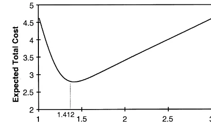
Let k* be the value of the process mean that minimizes EPC(k). An example of EPC(k) is given in Fig. 1, where a"1,b"1.2, and c
r"5. Note
that the function is unimodal withk*"1.412, and the nonconforming rate associated withk*is 0.98%.
Fig. 1. The expected per-item total cost as a function of process mean.
For a given¹and<, we consider two mutually exclusive and exhaustive events. In event A, the cycle time,¹, is less than or equal to the time of the shift to the out-of-control state,<(i.e.,¹)<). In this situation, since the manufacturing process is always in control during the entire cycle, the ex-pected per-item total cost is EPC(k
0) and the condi-tional expected total cost in a cycle is given by
ETC(k
0D¹)<)"r¹EPC(k0).
In eventB, the cycle time is longer than the process shift time. That is, the process is out of control prior to the end of the production run. The EPC asso-ciated with the items produced between times 0 and <is EPC(k
0) and that between times<and¹ is EPC(k
1). As a result, the conditional total expected cost in a cycle is
ETC(k
0D¹'<)"(r<)EPC(k0)
#r(¹!<)EPC(k 1).
IfK is de"ned as the setup cost for the process, then by using the above results, the unconditional total expected cost per cycle is obtained by
ETC"
T
P
0 ETC(k
0D¹'<)je~jvdv
#
=
P
TETC(k
and the unit time expected total cost is
EUC"ETC/¹.
The objective is to determine the optimal process mean,uH0, and cycle time,¹H, that minimize EUC. It can be shown that EUC is given by
EUC"
A
rj*EPC(k0)(1!ejT)
#r¹EPC(k
1)#K)
N
¹ (3)where *EPC(k0)"EPC(k0)!EPC(k1), which is the per-item cost di!erence between the in-control and out-of-control states. Since EPC(k
1) is con-stant, it is evident that the optimal value fork
0isk* which minimizes EPC(k).
The"rst derivative condition,LEUC/L¹"0, for
the optimal cycle time is equivalent to
e~jT(1#j¹)"1# jK
r*EPC(k
0)
. (4)
Since e~jT(1#j¹) is equal to 1 when¹"0 and is a strictly decreasing function of¹, there is a unique solution to (4) when*EPC(k
0)(0. Therefore, let-tingk
0"uH, the optimal cycle time,¹H, is obtained
by solving (4). Because of the complexity of expres-sion (4), a one-dimenexpres-sional search procedure can be used to"nd¹H. For convenience, let EUC*denote the unit time cost associated with the optimal solutionuHand¹H.
Example 1. Consider a product that requires at least 1.0 mg of main content in each item produced. Any item that is less than 1.0 mg is considered nonconforming and results in a loss (i.e., a penalty cost re#ecting material and production opportun-ity costs) of$5. Because of variation in the produc-tion process, the content of an item produced by the process follows a normal distribution with a con-stant standard deviation of 0.2 mg. Furthermore, the process may go out-of-control any time during the course of production. When this occurs, the process mean shifts to 1.2 mg. Assume the arrival of the out-of-control state follows an exponential dis-tribution with an arrival rate of 0.04 per unit time. The production rate is 100 items per unit time. The
setup cost per production run is$150 and the"xed and variable production costs are a"$1 and
b"$1.2 per item, respectively.
A MATLAB [38] program was written to imple-ment the solution procedure.1For Example 1, the optimal production cycle time is ¹H"16.07 and the optimal process mean isuH"1.412 mg with an average unit time cost of EUC*"$300.176. The nonconforming rate associated with the process mean is 0.98% and the average cost of producing an item is$2.793. On the other hand, the noncon-forming rate when the process is out-of-control increases to 15.9% and the average cost of produ-cing an item increases to$3.233. If the process does not go out-of-control during the cycle, the unit time cost would be$288.621. Comparing this cost with that of the optimal solution, it is apparent the process is in control a relatively high proportion of the run time.
3. Process improvements
In this section, the cost implications of three types of process improvement actions are assessed: reducing the setup cost, reducing the arrival rate of the out-of-control state, and reducing the process variance. Example 1 is used as the baseline in the study.
3.1. Setup cost
To study the e!ect of setup cost on the optimal solution, we obtain the optimal solutions for se-lected values of the setup cost, ranging from 90 to 160. As would be expected, as the setup cost is decreased, the cycle time and the EUC decrease. We found that the relationships between the cycle time and setup cost and between the EUC and the setup cost are approximately linear. Furthermore, when the setup cost is reduced, for example, from 160 to 90 (a 43.8% reduction), the EUC is reduced by only about 1.7%. Although this result implies
that the optimal solution is robust with respect to
K, it also suggests that improvements in setup cost may not signi"cantly reduce producer's cost. Per-centage improvements are constrained because a large proportion of EUC consists of production costs that are simply not a!ected by the setup policy. In order to more accurately re#ect the
bene-"t of an investment in reducing the setup cost, we
build upon the approaches of Golhar and Pollock [11] and Al-Sultan and Al-Fawzan [12] and pro-pose the following method.
Since EPC(k*) is the minimum expected cost of producing an item, then if the process stays in control all the time, the smallest possible unit time cost is
EUC
1"EPC(kH)r. If EUC
1 is taken a baseline cost for comparison purposes, then the maximum cost reduction due to an improvement (i.e., decrease) in the setup cost is
*EUC"EUCH!EUC
1,
which will the basis for evaluating any bene"t of an investment in reducing setup cost.
To determine the investment level that yields optimal setup cost reduction, we take an approach which is similar to but slightly di!erent from Porteus'[39,3]. Suppose an investment ofC(K) can reduce the setup cost fromK
0to K. Consider the logarithmic form discussed by Porteus: the cost to improve the setup cost fromK
0toKis
C(K)"A!Bln(K) for 0(K(K
0.
An important property of this function is that it costs a "xed amount to reduce the setup cost by a given proportion. For example, assume it costs
gdollars to reduce the setup cost fromK0"150 by
10%, C(K)"A!Bln(135). Since C(150)"0, we
"nd B"!g/ln(0.9) and A"Bln(K
0). Let
g"$200, then B"1898.24 and A"9511.39.
The cost of changing K to 150]0.9 ("135) is C(135)"$200. If we want to reduce the setup cost by another 10% (from K"135),
C(K)"A!Bln(121.5). The incremental cost,
C(121.5)!C(135), is still$200.
Note that the decision to reduce setup cost rep-resents a one time investment. In order to
incorpor-ate this investment into EUC, we introduce the concept of a planning horizon. LetHbe the length of time that the producer will bene"t from the investment. Using undiscounted costs, the total cost for planning horizonHis
TC"HEUC#A!Bln(K),
and the average total cost per unit time is
ATC"EUC#A!Bln(K)/H. (5)
The "rst derivative of ATC with respect to K is
given by
LATC
LK "
1
¹!
B
HK,
which leads to¹"HK/B. Therefore, a one-dimen-sional search onK where¹"HK/Bcan"nd the optimalKand¹which minimize ATC.
Example 1 (Continued). Assume H"600 and the cost function associated with the setup cost reduc-tion (5). If the other parameters remain the same as in Example 1, the optimal solution is to invest a total of$4,697 to reduce the setup cost to$12.63 (which is 8.43% of the original value.) This invest-ment results in a cycle time of 3.99. The average total cost per unit time is $293.62, which now includes EUC"$285.79 plus an investment of
3.2. Arrival rate of the out-of-control state
The"rst derivative of EUC with respect tojis
LEUC
The second derivative of EUC with respect tojis
!j2¹e~jT, thus (1#j¹)e~jTis a decreasing func-tion ofj. Furthermore, since (1#j¹)e~jT!1"0
when j"0, (1#j¹)e~jT!1(0 for j'0.
Because *EPC(k
0)(0,LEUC/Lj'0, it appears EUC can be reduced by an investment in reducing
j.
Consider again the logarithmic form of the cost improvement function. However, this time applied to reducingj. The cost to improve the arrival rate of the out-of-control state fromj
0tojis
C(K)"A!Bln(j) for 0(j(j
0.
Adding this cost function to EUC, the average cost per unit time is
ATC"EUC#A!Bln((j)
H .
The "rst derivative of ATC with respect to j is
given as
and that with respect to¹is given as
LATC mal cycle time is determined by¹"HK/B, which is exactly the same relationship between the cycle time, planning horizon, and the setup cost found in the last subsection, dealing with the setup cost improvement. Consequently, the optimalj corre-sponding to the optimal ¹value can be obtained by numerically solvingLATC/Lj"0.
Substituting¹"HK/Bin expression (3), we ob-tain the following expression for EUC:
EUC" rB
(jKH)[1!e~(jK)H@B]*EPC(k0)#
B
H.
From the last expression, it is apparent that the e!ect of a percentage reduction injon EUC is the same as that of the same percentage reduction inK. Consequently, the cost bene"ts of improving the setup cost and the arrival rate of the out-of-control state are the same.
Example 1(Continued). Suppose the cost of reduc-ing the arrival rate of the out-of-control state from the current level (j0"0.04) by 10% is $200. The logarithmic form of the cost function is
C(j)"!6110.21!1898.244 ln(j).
WhenH"600, the optimal solution is to invest
$4697 to reducejto 0.0034, which is about 8.4% of the original value before improvement. This invest-ment results in a cycle time of 47.41. As discussed, the cost bene"t of reducingjis equivalent to that of reducing K. The average cost per unit time is
$293.62, which includes EUC"$285.79 plus an investment of$7.83 to reduce the occurrence rate of the out-of-control state. The average cost per unit time amounts to a 31.4% reduction in*EUC.
To study the e!ects of planning horizon on the investment strategy for reducing j, optimal solu-tions were obtained for selected values of H, ranging from 400 to 1200. As expected, the bene"ts of improvement are found identical to those asso-ciated with setup cost improvement. We also found that the total investment,C(j), increases approxi-mately linearly as H increases. The results also show that the optimaljvalue decreases rapidly as
Hincreases. Note that a smallerjimplies that the process will stay in control for a longer time, and therefore the cycle time should become larger. Since the optimal cycle is determined by¹"HK/B, the cycle time increases linearly asHincreases. There-fore, it is expected that the e!ect of improvement is larger for a longer planning horizon. Furthermore, similar to the e!ects of setup cost improvement, when the planning horizon increases from 400 to 1200, the improvement increases almost linearly from 16% to 55%. Although formal proof is not given here, it is evident that whenHbecomes in" -nitely large,jwill approach 0. Under these condi-tions, the process will remain essentially in-control for the duration of the planning horizon and the optimal strategy is to setk
process continuously (i.e.,¹"R). The cost asso-ciated with this situation is EUC
1"$279.29 and
the percent improvement is 100%.
3.3. Processvariance
Recall that in determining the appropriatek*to minimize EPC(k),k*cannot be set at¸because of the existence of variation in the process,p2. Since
k*must be greater than¸, excess material costs are absorbed as a necessary condition to reducing the nonconforming rate. Ifp2can be reduced, the pro-cess mean can be set closer to¸. This will lead to a lower nonconforming rate, a lower material cost, or both.
We again use the logarithmic form for the cost function of reducing p: The cost to reduce the process standard deviation fromp
0to pis
C(p)"A!Bln(p) for 0(p(p0.
As before, the average total cost per unit time is
ATC"EUC#A!Bln(p)
H .
When minimizing ATC, k
0 becomes a decision variable because pis also a decision variable (i.e., the optimal value of k
0 changes as other model parameters change). Because of the complexity of
the"rst derivatives of ATC with respect tokandp,
the optimal solution is obtained by direct search. To ensure optimality, multiple starting points are used and the"rst derivative condition is tested for the optimal ¹, LE;C/L¹"0. We found that the results of sample problems appear satisfactory and make intuitive sense.
Example 1 (Continued). Suppose that the cost to reduce the arrival rate of the out-of-control state from the current level (p0 "0.2 mg) by 10% is
$200. The improvement cost function is
C(p)"!3055.11!1898.244 ln(p).
Note that when p changes, the standardized dis-tance between ¸ andk
1changes. To ensure con-stant relationships between¸andk
1, we letk1be
determined by¸#p. Furthermore, whenpcan be reduced, we modify the minimum production cost that is not a!ected byp. This cost is the unit time production cost whenp is equal to 0. Under this situation, the process mean is set at¸and yields the following minimum cost:
EUC
2"EPC(¸)r.
Thus, the maximum improvement due to a reduc-tion in the process standard deviareduc-tion is
*EUC"EUCH!EUC
2,
which is used to evaluate any bene"ts of reducingp. Consider again a planning horizonH"600. The optimal solution is to invest$5783 to improve (i.e., reduce) the process standard deviation to 0.0095, which is about 4.75% of the original value. The process mean is set at 1.0305, which is very close to the lower limit ¸. The unit production costs at
k
0 and k1 are $2.2399 and $3.0047, respectively. The cycle time is 11.51, which is smaller than that under no improvement inp. The average total cost per unit time associated with the optimal solution is
$261.85 and EUC
2is $220. As a result, *EUC" 80.18, and the percent improvement due to a reduc-tion in process variance is 47.80%.
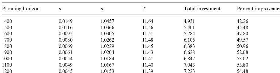
To study the e!ects ofHon the optimal solution, we obtain solutions under selected values of H, ranging from 400 to 1200. Because the results in-volve several decision variables and costs, Table 1 (instead of graphs) is used to present the results. As expected, whenH is larger, a larger investment is made, resulting in smallerp andk
0. Furthermore, whenH is larger, the di!erence between EPC(k
0) and EPC(k
Table 1
The results associated with improvement on process variation.
Planning horizon p k ¹ Total investment Percent improvement
400 0.0149 1.0457 11.64 4,931 42.26
500 0.0116 1.0366 11.56 5,401 45.48
600 0.0095 1.0305 11.51 5,784 47.80
700 0.0080 1.0262 11.48 6,105 49.57
800 0.0069 1.0229 11.45 6,383 50.96
900 0.0061 1.0204 11.43 6,628 52.08
1000 0.0054 1.0184 11.41 6,847 53.02
1100 0.0049 1.0167 11.40 7,043 53.80
1200 0.0045 1.0153 11.39 7,223 54.48
4. Discussion
In this paper, we examined process improvement alternatives for a container-"lling process. Three types of improvement actions for modifying model parameters are considered: reducing the process setup cost, reducing the arrival rate of the out-of-control state, and reducing the process variance. It is assumed that these process parameters can be changed with a one-time investment. In studying the optimal investment strategy, the concept of a planning horizon is introduced and de"ned as the length of time that the bene"t from an improve-ment obtains. Models are formulated to determine the optimal investment that minimizes the unit time expected cost over the planning horizon. Numerical analyses are used to study the relationship between the optimal investment strategy, the process para-meters and the length of the planning horizon.
In this paper, it is assumed that the process mean
is"xed ("k
1) when the process is out-of-control. It is germane to note that the literature describes an alternative state shift mechanism in which the pro-cess mean drops from the initial level,k
0, by a"xed amount*k(i.e., the process mean isk
0!*kwhen the process is out-of-control). Under this assump-tion,LEUC/LT is negative when*EPC(k
0)'0 (see the discussion relating to expression (4)). As a re-sult, the optimal strategy in this situation is to set
k
0"k*#*kand let¹"R. In other words, the
strategy is to wait for the out-of-control state (in fact, the best process condition) to occur and oper-ate the process inde"nitely! The EUC associated
with this strategy is limit
T?=EUC"rEPC(kH). It
appears that this approach (and the corresponding assumptions) may be problematic.
The model structure presented in this paper pro-vides a useful framework for future research on several interesting issues related to the assumptions used in this paper. In particular, the following three extensions are possible. First, the model can be easily modi"ed to consider the situation in which quantity discounts are available for raw material purchasing. The second extension is to incorporate production process deterioration in addition to random failure into the model. For example, the Weibull distribution may be used to replace the exponential distribution. The third extension is to consider a multiple-level "lling process in which several raw materials are added in di!erent stages. However, this issue could be very complicated when the product conformance is jointly deter-mined by the amounts of several raw materials and process improvement may be considered for di! er-ent stages of the"lling process.
References
[1] C.C. Harwood, G.R. Pieters, How to manage quality im-provement, Quality Progress 23 (3) (1990) 45}48. [2] R.P. Mohanty, N. Dahanayka, Process improvement:
Evaluation of methods, Quality Progress 22 (9) (1989) 45}48.
[4] M.J. Rosenblatt, H.L. Lee, Economic production cycles with imperfect production processes, IIE Transactions 18 (1986) 48}55.
[5] C. Fine, E.L. Porteus, Dynamic process improvement, Operations Research 37 (1989) 580}591.
[6] G. Keller, H. Noori, Impact of investing in quality im-provement on the lot size model, Omega 16 (1988) 595}601.
[7] L. Gong, J. Pruett, K. Tang, A Markovian model for process setup and improvement, Naval Research Logistics 44 (1997) 383}400.
[8] W.I. Zangwill, From EOQ toward ZI, Management Science 33 (10) (1987) 1209}1223.
[9] G. Taguchi, Introduction to Quality Evaluation and Quality Control, Japanese Standards Association, Tokyo, Japan, 1978.
[10] J. Roan, L. Gong, K. Tang, Process mean determination under constant material supply, European Journal of Operational Research 99 (2) (1997) 353}365.
[11] D.Y. Golhar, S.M. Pollock, Cost savings due to variance deduction, IIE Transactions 24 (1) (1992) 89}92. [12] K.S. Al-Sultan, M.A. Al-Fawzan, Variance reduction in
a process with random linear drift, International Journal of Production Research 35 (6) (1997) 1523}1534. [13] C. Fine, A quality control model with learning e!ects,
Operations Research 36 (1988) 437}444.
[14] C. Tapiero, Production learning and quality control, IIE Transactions 19 (4) (1987) 362}370.
[15] D.C. Bettes, Finding an optimal target value in relation to a"xed lower limit and an arbitrary upper limit, Applied Statistics 11 (1962) 202}210.
[16] W.G. Hunter, C.P. Kartha, Determining the most pro" t-able target value for a production process, Journal of Quality Technology 9 (1977) 176}181.
[17] L.S. Nelson, Best target value for a production process, Journal of Quality Technology 10 (1978) 88}89. [18] O. Carlsson, Determining the most pro"table process level
for a production process under di!erent sales conditions, Journal of Quality Technology 23 (1984) 44}47. [19] S. Bisgaard, W.G. Hunter, L. Pallesen, Economic selection
of quality of manufactured product, Technometrics 26 (1984) 9}18.
[20] D.Y. Golhar, S.M. Pollock, Determination of the optimal process mean and the upper limit for a canning problem, Journal of Quality Technology 20 (1988) 188}192. [21] R.L. Schmidt, P.E. Pfeifer, Economic selection of the mean
and upper limit for a canning problem with limited capa-city, Journal of Quality Technology 23 (1991) 312}317. [22] T.O. Boucher, M. Jafari, The optimum target value for
single"lling operations with quality sampling plans, Jour-nal of Quality Technology 23 (1991) 44}47.
[23] K.S. Al-Sultan, An algorithm for the determination of the optimal target values for two machines in series with quality sampling plans, International Journal of Produc-tion Research 12 (1) (1994) 37}45.
[24] M.F.S. Pulak, K.S. Al-Sultan, On the optimum targeting for a single "lling operation with rectifying inspection, Working paper, Department of Systems Engineering, King Fahd University of Petroleum and Minerals, Saudi Arabia, 1995.
[25] K. Tang, J. Lo, Determination of the optimal process mean when inspection is based on a correlated variable, IIE Transactions 25 (3) (1993) 66}72.
[26] J. Liu, K. Tang, Y. Chun, Container-"lling problem under capacity constraints, in: K.S. Al-Sultan, M.A. Rahim (Eds.), Optimization in Quality Control, Kluwer Academic Publishers, Boston, Massachusetts, 1997, pp. 215}229.
[27] L. Gong, J. Roan, K. Tang, Process mean determination with quantity discounts in raw material cost, Decision Sciences (1999), forthcoming.
[28] M.A. Rahim, R.S. Lashkari, Optimal decision rules for determining the length of production run, Computers and Industrial Engineering 9 (1985) 195}202.
[29] I.N. Gibra, Optimal control of processes subject to linear trends, Journal of Industrial Engineering 18 (1) (1967) 35}41.
[30] H.A. Taha, A policy for determining the optimal cycle length for cutting tool, Journal of Industrial Engineering 17 (3) (1966) 157}162.
[31] F.J. Arcelus, P.K. Banerjee, Selection of the most economi-cal production plan in a tool-wear process, Technometrics 27 (4) (1985) 433}437.
[32] M.A. Rahim, P.K. Banerjee, Optimal production run for a process with random linear drift, Omega 16 (4) (1988) 347}351.
[33] H. Schneider, K. Tang, C. O'Cinneide, Optimal control of a production process subject to random deterioration, Operations Research 38 (6) (1990) 1116}1122.
[34] F.J. Arcelus, P.K. Banerjee, R. Chandra, Optimal produc-tion run for a normally distributed quality characteristic exhibiting non-negative shifts in process mean and variance, IIE Transactions 14 (1982) 90}98.
[35] K. Tang, J. Tang, Design of screening procedures: a review, Journal of Quality Technology 26 (1994) 209}226.
[36] K.S. Al-Sultan, M.A. Rahim, Economic selection of process parameters: A literature survey, Working paper, Department of Systems Engineering, King Fahd University of Petroleum and Minerals, Saudi Arabia, 1994.
[37] M.A. Rahim, K.S. Al-Sultan, Some contemporary ap-proaches to optimization models in process control, in: K.S. Al-Sultan, M.A. Rahim (Eds.), Optimization in Qual-ity Control, Kluwer Academic Publishers, Boston, MA, 1997.
[38] MATLAB, Optimization Toolbox, The Mathworks Inc., Natick, MA, 1982.