Contents
1. Learning Outcome Statements (LOS)
2. Study Session 8—Applications of Economic Analysis to Portfolio Management 1. Reading 16: Capital Market Expectations
1. Exam Focus
2. Module 16.1: Formulating Capital Market Expectations
3. Module 16.2: Statistical Tools and Discounted Cash Flow Models 4. Module 16.3: Risk Premiums, Financial Equilibrium, and Surveys 5. Module 16.4: The Business Cycle
6. Module 16.5: Monetary Policy and Interest Rates 7. Module 16.6: The Trend Rate of Growth
8. Module 16.7: International Considerations 9. Module 16.8: Market Forecasting
10. Module 16.9: Exchange Rate Forecasting 11. Module 16.10: Comprehensive Example 12. Key Concepts
13. Answer Key for Module Quizzes 2. Reading 17: Equity Market Valuation
1. Exam Focus
2. Module 17.1: Cobb-Douglas Production Function 3. Module 17.2: Dividend Discount Models
4. Module 17.3: Top-Down VS. Bottom-Up 5. Module 17.4: Fed Model
6. Module 17.5: The Yardeni Model 7. Module 17.6: CAPE
8. Module 17.7: Q-Models 9. Key Concepts
10. Answer Key for Module Quizzes 3. Topic Assessment: Economic Analysis
4. Topic Assessment Answers: Economic Analysis
5. Study Session 9—Asset Allocation and Related Decisions in Portfolio Management (1)
1. Reading 18: Introduction to Asset Allocation 1. Exam Focus
2. Module 18.1: Economic Balance Sheet
3. Module 18.2: Approaches to Asset Allocation
4. Module 18.3: Allocation by Asset Class or Risk Factor 5. Module 18.4: Example: Strategic Asset Allocation 6. Module 18.5: Other Approaches and Issues
7. Key Concepts
8. Answer Key for Module Quizzes 2. Reading 19: Principles of Asset Allocation
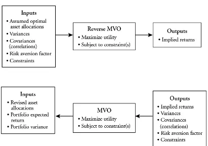
2. Module 19.1: Basic Mean-Variance Optimization
3. Module 19.2: Reverse Optimization, Black Litterman, Resampling, and Other Approaches
4. Module 19.3: Example
5. Module 19.4: Issues for Individuals
6. Module 19.5: A Risk Budgeting Approach 7. Module 19.6: An ALM Approach
8. Module 19.7: Goals-Based and Miscellaneous Approaches 9. Module 19.8: Rebalancing Policy
10. Key Concepts
11. Answer Key for Module Quizzes
6. Study Session 10—Asset Allocation and Related Decisions in Portfolio Management (2)
1. Reading 20: Asset Allocation With Real-World Constraints 1. Exam Focus
2. Module 20.1: Real World Issues
3. Module 20.2: Adjusting the Strategic asset allocation 4. Module 20.3: Behavioral Issues
5. Key Concepts
6. Answer Key for Module Quizzes
2. Reading 21: Currency Management: An Introduction 1. Exam Focus
2. Module 21.1: Managing Currency Exposure
3. Module 21.2: Active Strategies: Fundamentals and Technical 4. Module 21.3: Active Strategies: Carry and Volatility Trading 5. Module 21.4: Implementation and Forwards
6. Module 21.5: Implementation and Options 7. Key Concepts
8. Answer Key for Module Quizzes 7. Topic Assessment: Asset Allocation
8. Topic Assessment Answers: Asset Allocation
9. Study Session 11—Fixed-Income Portfolio Management (1)
1. Reading 22: Fixed-Income Portfolio Management: Introduction 1. Exam Focus
2. Module 22.1: Role of Fixed Income 3. Module 22.2: Modeling Return
4. Module 22.3: Leverage and Tax Issues 5. Key Concepts
6. Answer Key for Module Quizzes
2. Reading 23: Liability-Driven and Index-Based Strategies 1. Exam Focus
2. Module 23.1: LDI, Basics
3. Module 23.2: Managing a Duration Gap 4. Module 23.3: Advanced strategies 5. Module 23.4: Risks
7. Module 23.6: Introduction: Bullet, Ladder, Barbell 8. Key Concepts
9. Answer Key for Module Quizzes
10. Study Session 12—Fixed-Income Portfolio Management (2) 1. Reading 24: Yield Curve Strategies
1. Exam Focus
2. Module 24.1: Introduction and Strategies for an Unchanged Curve 3. Module 24.2: Strategies for Changing Yield Curves
4. Module 24.3: Adjusting Convexity 5. Module 24.4: Carry Trades
6. Module 24.5: Determining an Optimal Strategy
7. Module 24.6: Using Derivatives to Implement a Yield Curve Strategy 8. Module 24.7: Using Key Rate Durations to Determine Optimal
Strategy
9. Module 24.8: Inter-Market Curve Strategies and Conclusion 10. Key Concepts
11. Answer Key for Module Quizzes
2. Reading 25: Fixed-Income Active Management: Credit Strategies 1. Exam Focus
2. Module 25.1: IG vs. HY and Measuring Spread 3. Module 25.2: Top-Down and Bottom-Up
4. Module 25.3: Liquidity, Tail, and International Risks 5. Module 25.4: Structured Instruments
6. Key Concepts
7. Answer Key for Module Quizzes
11. Topic Assessment: Fixed-Income Portfolio Management
STUDY SESSION 8
The topical coverage corresponds with the following CFA Institute assigned reading:
16. Capital Market Expectations The candidate should be able to:
a. discuss the role of, and a framework for, capital market expectations in the portfolio management process. (page 1)
b. discuss challenges in developing capital market forecasts. (page 2)
c. demonstrate the application of formal tools for setting capital market expectations, including statistical tools, discounted cash flow models, the risk premium
approach, and financial equilibrium models. (page 7)
d. explain the use of survey and panel methods and judgment in setting capital market expectations. (page 19)
e. discuss the inventory and business cycles and the effects that consumer and business spending and monetary and fiscal policy have on the business cycle. (page 20)
f. discuss the effects that the phases of the business cycle have on short-term/long-term capital market returns. (page 21)
g. explain the relationship of inflation to the business cycle and the implications of inflation for cash, bonds, equity, and real estate returns. (page 24)
h. demonstrate the use of the Taylor rule to predict central bank behavior. (page 28) i. interpret the shape of the yield curve as an economic predictor and discuss the
relationship between the yield curve and fiscal and monetary policy. (page 31) j. identify and interpret the components of economic growth trends and demonstrate
the application of economic growth trend analysis to the formulation of capital market expectations. (page 32)
k. explain how exogenous shocks may affect economic growth trends. (page 34) l. identify and interpret macroeconomic, interest rate, and exchange rate linkages
between economies. (page 36)
m. discuss the risks faced by investors in emerging-market securities and the country risk analysis techniques used to evaluate emerging market economies. (page 37) n. compare the major approaches to economic forecasting. (page 38)
o. demonstrate the use of economic information in forecasting asset class returns. (page 40)
p. explain how economic and competitive factors can affect investment markets, sectors, and specific securities. (page 40)
q. discuss the relative advantages and limitations of the major approaches to forecasting exchange rates. (page 44)
r. recommend and justify changes in the component weights of a global investment portfolio based on trends and expected changes in macroeconomic factors. (page 46)
The topical coverage corresponds with the following CFA Institute assigned reading:
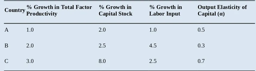
a. explain the terms of the Cobb-Douglas production function and demonstrate how the function can be used to model growth in real output under the assumption of constant returns to scale. (page 61)
b. evaluate the relative importance of growth in total factor productivity, in capital stock, and in labor input given relevant historical data. (page 63)
c. demonstrate the use of the Cobb-Douglas production function in obtaining a discounted dividend model estimate of the intrinsic value of an equity market. (page 66)
d. critique the use of discounted dividend models and macroeconomic forecasts to estimate the intrinsic value of an equity market. (page 66)
e. contrast top-down and bottom-up approaches to forecasting the earnings per share of an equity market index. (page 69)
f. discuss the strengths and limitations of relative valuation models. (page 72) g. judge whether an equity market is under-, fairly, or over-valued using a relative
泽稷网校2017-2018年最新CFA一级二级考点汇总中 文版根据CFA最新考纲编写,比看notes还有效率
扫码关注以上微信公众号:CFAer,回复
【资料】即可免费获取全套资源!此活动
永久有效!资料会常年实时更新!绝对全
面!
【CFA万人微信群】
需要加入我们CFA全球考友微信群的请添加CFA菌的微信号:374208596,备注需要加哪些群~或直接 扫下方CFA菌菌二维码即可~
所有人均先加入CFA全球考友总群再根据您的需求加入其他分群~
(2017年12月,2018年6打卡签到监督群,一级、二级、三级分群、上海、武汉、北京、成都、南 京、杭州、广州深圳、香港、海外等分群)!
备考资料、学霸考经、考试资讯免费共享!交流、答疑、互助应有尽有!快来加入我们吧!群数量 太多,文件中只是部分展示~有困难的话可以随时咨询我哦!
全套资源获取方式随新考 季更新,永久有效!
2017-2018年泽稷网校CFA视频音频课程及指南
除CFA资料外赠送金融、财会技能视频包+热门书籍 +1000G考证资料包
备考CFA的8大最有效资料和工具 教材/notes/核心词汇手册/考纲及解析手册/计算器讲 解、历年全真模拟题/真题/道德手册/QuickSheet/等等
史上最全的学霸学渣党CFA考经笔记分享
让你CFA备考路上不再孤独!不再艰难!
PD F里 所 有 资 料 扫 码 获 得
【CFA免费资料共享QQ群:526307508】
STUDY SESSION 9
The topical coverage corresponds with the following CFA Institute assigned reading:
18. Introduction to Asset Allocation The candidate should be able to:
a. prepare an economic balance sheet for a client and interpret its implications for asset allocation. (page 93)
b. compare the investment objectives of asset-only, liability-relative, and goals-based asset allocation approaches. (page 94)
c. contrast concepts of risk relevant to asset-only, liability-relative, and goals-based asset allocation approaches. (page 96)
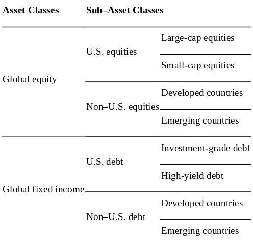
d. explain how asset classes are used to represent exposures to systematic risk and discuss criteria for asset class specification. (page 97)
e. explain the use of risk factors in asset allocation and their relation to traditional asset class–based approaches. (page 98)
f. select and justify an asset allocation based on an investor’s objectives and constraints. (page 99)
g. describe the use of the global market portfolio as a baseline portfolio in asset allocation. (page 102)
h. discuss strategic implementation choices in asset allocation, including
passive/active choices and vehicles for implementing passive and active mandates. (page 103)
i. discuss strategic considerations in rebalancing asset allocations. (page 105)
The topical coverage corresponds with the following CFA Institute assigned reading:
19. Principles of Asset Allocation The candidate should be able to:
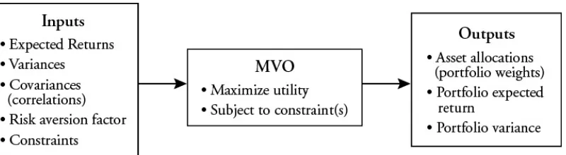
a. describe and critique the use of mean–variance optimization in asset allocation. (page 115)
b. recommend and justify an asset allocation using mean–variance optimization. (page 122)
c. interpret and critique an asset allocation in relation to an investor’s economic balance sheet. (page 125)
d. discuss asset class liquidity considerations in asset allocation. (page 126) e. explain absolute and relative risk budgets and their use in determining and
implementing an asset allocation. (page 127)
f. describe how client needs and preferences regarding investment risks can be incorporated into asset allocation. (page 129)
g. discuss the use of Monte Carlo simulation and scenario analysis to evaluate the robustness of an asset allocation. (page 125)
h. describe the use of investment factors in constructing and analyzing an asset allocation. (page 129)
j. describe and evaluate characteristics of liabilities that are relevant to asset allocation. (page 131)
k. discuss approaches to liability-relative asset allocation. (page 132) l. recommend and justify a liability-relative asset allocation. (page 132)
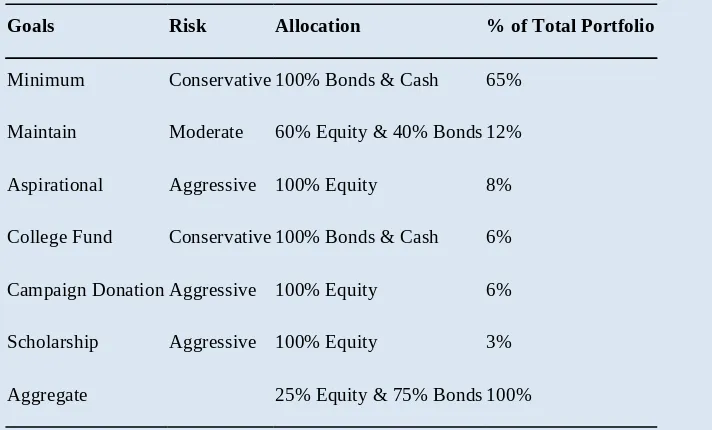
m. recommend and justify an asset allocation using a goals-based approach. (page 134)
STUDY SESSION 10
The topical coverage corresponds with the following CFA Institute assigned reading:
20. Asset Allocation with Real-World Constraints The candidate should be able to:
a. discuss asset size, liquidity needs, time horizon, and regulatory or other considerations as constraints on asset allocation. (page 145)
b. discuss tax considerations in asset allocation and rebalancing. (page 151) c. recommend and justify revisions to an asset allocation given change(s) in
investment objectives and/or constraints. (page 154)
d. discuss the use of short-term shifts in asset allocation. (page 156)
e. identify behavioral biases that arise in asset allocation and recommend methods to overcome them. (page 158)
The topical coverage corresponds with the following CFA Institute assigned reading:
21. Currency Management: An Introduction The candidate should be able to:
a. analyze the effects of currency movements on portfolio risk and return. (page 170) b. discuss strategic choices in currency management. (page 174)
c. formulate an appropriate currency management program given financial market conditions and portfolio objectives and constraints. (page 177)
d. compare active currency trading strategies based on economic fundamentals, technical analysis, carry-trade, and volatility trading. (page 181)
e. describe how changes in factors underlying active trading strategies affect tactical trading decisions. (page 186)
f. describe how forward contracts and FX (foreign exchange) swaps are used to adjust hedge ratios. (page 187)
g. describe trading strategies used to reduce hedging costs and modify the risk–return characteristics of a foreign-currency portfolio. (page 193)
h. describe the use of cross-hedges, macro-hedges, and minimum-variance-hedge ratios in portfolios exposed to multiple foreign currencies. (page 196)
STUDY SESSION 11
The topical coverage corresponds with the following CFA Institute assigned reading:
22. Introduction to Fixed-Income Portfolio Management The candidate should be able to:
a. discuss roles of fixed-income securities in portfolios. (page 217)
b. describe how fixed-income mandates may be classified and compare features of the mandates. (page 220)
c. describe bond market liquidity, including the differences among market sub-sectors, and discuss the effect of liquidity on fixed-income portfolio management. (page 222)
d. describe and interpret a model for fixed-income returns. (page 224)
e. discuss the use of leverage, alternative methods for leveraging, and risks that leverage creates in fixed-income portfolios. (page 227)
f. discuss differences in managing fixed-income portfolios for taxable and tax exempt investors. (page 230)
The topical coverage corresponds with the following CFA Institute assigned reading:
23. Liability-Driven and Index-Based Strategies The candidate should be able to:
a. describe liability-driven investing. (page 237)
b. evaluate strategies for managing a single liability. (page 238)
c. compare strategies for a single liability and for multiple liabilities, including alternative means of implementation. (page 246)
d. evaluate liability-based strategies under various interest rate scenarios and select a strategy to achieve a portfolio’s objectives. (page 252)
e. explain risks associated with managing a portfolio against a liability structure. (page 258)
f. discuss bond indexes and the challenges of managing a fixed-income portfolio to mimic the characteristics of a bond index. (page 259)
g. compare alternative methods for establishing bond market exposure passively. (page 262)
h. discuss criteria for selecting a benchmark and justify the selection of a benchmark. (page 264)
STUDY SESSION 12
The topical coverage corresponds with the following CFA Institute assigned reading:
24. Yield Curve Strategies The candidate should be able to:
a. describe major types of yield curve strategies. (page 276, 277) b. explain how to execute a carry trade. (page 276, 281)
c. explain why and how a fixed-income portfolio manager might choose to alter portfolio convexity. (page 276, 277, 279)
d. formulate a portfolio positioning strategy given forward interest rates and an interest rate view. (page 284)
e. explain how derivatives may be used to implement yield curve strategies. (page 277, 287)
f. evaluate a portfolio’s sensitivity to a change in curve slope using key rate durations of the portfolio and its benchmark. (page 291)
g. discuss inter-market curve strategies. (page 294)
h. construct a duration-neutral government bond portfolio to profit from a change in yield curve curvature. (page 292)
i. evaluate the expected return and risks of a yield curve strategy. (page 297)
The topical coverage corresponds with the following CFA Institute assigned reading:
25. Fixed-Income Active Management: Credit Strategies The candidate should be able to:
a. describe risk considerations in investment-grade and high-yield corporate bond portfolios. (page 306)
b. compare the use of credit spread measures in portfolio construction. (page 309) c. discuss bottom-up approaches to credit strategies. (page 312)
d. discuss top-down approaches to credit strategies. (page 312, 316)
e. discuss liquidity risk in credit markets and how liquidity risk can be managed in a credit portfolio. (page 321)
f. describe how to assess and manage tail risk in credit portfolios. (page 322)
g. discuss considerations in constructing and managing portfolios across international credit markets. (page 323)
Video covering this content is available online.
The following is a review of the Applications of Economic Analysis to Portfolio Management principles designed to address the learning outcome statements set forth by CFA Institute. Cross-Reference to CFA Institute Assigned Reading #16.
READING 16: CAPITAL MARKET
EXPECTATIONS
Study Session 8
EXAM FOCUS
Combining capital market expectations with the client’s objectives and constraints leads to the portfolio’s strategic asset allocation. A variety of economic tools and techniques are useful in forming capital market expectations for return, risk, and correlation by asset class. Unfortunately, no one technique works consistently, so be prepared for any technique and its issues as covered here.
MODULE 16.1: FORMULATING CAPITAL MARKET
EXPECTATIONS
LOS 16.a: Discuss the role of, and a framework for, capital market expectations in the portfolio management process.
CFA® Program Curriculum, Volume 3, page 7
Capital market expectations can be referred to as macro expectations (expectations regarding classes of assets) or micro expectations
(expectations regarding individual assets). Micro expectations are most directly used in individual security selection. In other assignments, macro expectations are referred to as top-down while micro expectations are referred to as bottom-up.
Using a disciplined approach leads to more effective asset allocations and risk
management. Formulating capital market expectations is referred to as beta research because it is related to systematic risk. It can be used in the valuation of both equities and fixed-income securities. Alpha research, on the other hand, is concerned with earning excess returns through the use of specific strategies within specific asset groups. To formulate capital market expectations, the analyst should use the following 7-step process.
Step 1: Determine the specific capital market expectations needed according to the investor’s tax status, allowable asset classes, and time horizon. Time horizon is particularly important in determining the set of capital market expectations that are needed.
With the drivers of past performance established, the analyst can use these to forecast expected future performance as well as compare the forecast to past results to see if the forecast appears reasonable.
Step 3: Identify the valuation model used and its requirements. For example, a
comparables-based, relative value approach used in the United States may be difficult to apply in an emerging market analysis.
Step 4: Collect the best data possible. The use of faulty data will lead to faulty conclusions. The following issues should be considered when evaluating data for possible use:
Calculation methodologies. Data collection techniques. Data definitions.
Error rates.
Investability and correction for free float. Turnover in index components.
Potential biases.
Step 5: Use experience and judgment to interpret current investment conditions and decide what values to assign to the required inputs. Verify that the inputs used for the various asset classes are consistent across classes.
Step 6: Formulate capital market expectations. Any assumptions and rationales used in the analysis should be recorded. Determine that what was specified in Step 1 has been provided.
Step 7: Monitor performance and use it to refine the process. If actual performance varies significantly from forecasts, the process and model should be refined.
PROBLEMS IN FORECASTING
LOS 16.b: Discuss challenges in developing capital market forecasts.
CFA® Program Curriculum, Volume 3, page 13
As mentioned earlier, poor forecasts can result in inappropriate asset allocations. The analyst should be aware of the potential problems in data, models, and the resulting capital market expectations. Nine problems encountered in producing forecasts are (1) limitations to using economic data, (2) data measurement error and bias, (3) limitations of historical estimates, (4) the use of ex post risk and return measures, (5) non-repeating data patterns, (6) failing to account for conditioning information, (7) misinterpretation of correlations, (8) psychological traps, and (9) model and input uncertainty.
are often rebased over time (i.e., the base upon which they are calculated is changed). Although a rebasing is not a substantial change in the data itself, the unaware analyst could calculate changes in the value of the indices incorrectly if she does not make an appropriate adjustment.
2. There are numerous possible data measurement errors and biases.
Transcription errors are the misreporting or incorrect recording of information and are most serious if they are biased in one direction. Survivorship bias
commonly occurs if a manager or a security return series is deleted from the historical performance record of managers or firms. Deletions are often tied to poor performance and bias the historical return upward. Appraisal (smoothed)
data for illiquid and infrequently priced assets makes the path of returns appear smoother than it actually is. This biases downward the calculated standard
deviation and makes the returns seem less correlated (closer to 0) with more liquid priced assets. This is a particular problem for some types of alternative assets such as real estate. Rescaling the data based on underlying economic drivers can be used to leave the mean return unaffected but increase the variance.
3. The limitations of historical estimates can also hamper the formation of capital market expectations. The values from historical data must often be adjusted going forward as economic, political, regulatory, and technological environments
change. This is particularly true for volatile assets such as equity. These changes are known as regime changes and result in nonstationary data. For example, the bursting of the technology bubble in 2000 resulted in returns data that were markedly different than that from the previous five years. Nonstationarity would mean different periods in the time series have different statistical properties and create problems with standard statistical testing methods.
Historical data is the starting point for estimating the following capital market expectations: expected return, standard deviation, and correlations. However, it is not obvious how to select the time period of historical data. A long time period is preferable for several reasons.
It may be statistically required. To calculate historical covariance (and correlation), the number of data points must exceed the number of covariances to be calculated.
A larger data set (time period) provides more precise statistical estimates with smaller variance to the estimates.
As a related issue, if the time period is longer for a larger data set, the calculated statistics are generally less sensitive to the starting and ending points selected for the time period.
However, long time periods also create potential problems.
Financial Market Meltdown of 2008. 1) This creates nonstationarity, which invalidates many statistics calculated from time periods starting before and ending after the meltdown. 2) It forces the analyst to use judgment to decide whether the subperiod before or after the meltdown will be more relevant going forward.
It may mean the relevant time period is too short to be statistically significant.
It creates a temptation to use more frequent data, such as weekly data, rather than monthly data points in order to have a larger sample size.
Unfortunately, more frequent data points are often more likely to have missing or outdated values (this is called asynchronism) and can result in lower, distorted correlation calculations.
Two questions can be used to help resolve the issue of time period to select:
a. Is there a reason to believe the entire (longer) time period is not appropriate?
b. If the answer to the first question is yes, does a statistical test confirm there is a regime change and the point in the time series where it occurs?
If both answers are yes, the analyst must use judgment to select the relevant sub period.
PROFESSOR’S NOTE
I hope most candidates recognize the discussions above have been referring to many of the statistical testing issues covered at Level I and II. The focus here is not on performing such tests or even knowing which specific tests to use, but on recognizing times and ways testing can be relevant. Think of a senior portfolio manager who understands the larger issues and when to ask others with relevant technical skills to do further analysis. This is a common perspective at Level III.
4. Using ex post data (after the fact) to determine ex ante (before the fact) risk and return can be problematic. For example, suppose that several years ago investors were fearful that the Federal Reserve was going to have to raise interest rates to combat inflation. This situation would cause depressed stock prices. If inflation abated without the Fed’s intervention, then stock returns would increase once the inflation scenario passes. Looking back on this situation, the researcher would conclude that stock returns were high while being blind to the prior risk that investors had faced. The analyst would then conclude that future (ex ante) returns for stocks will be high. In sum, the analyst would underestimate the risks that equity investors face and overestimate their potential returns.
span of data chosen (time period bias). For example, small-cap U.S. stocks are widely thought to outperform large-cap stocks, but their advantage disappears when data from the 1970s and 1980s is excluded.
To avoid these biases, the analyst should first ask himself if there is any economic basis for the variables found to be related to stock returns. Second, he should scrutinize the modeling process for susceptibility to bias. Third, the analyst should test the discovered relationship with out-of-sample data to determine if the
relationship is persistent. This would be done by estimating the relationship with one portion of the historical data and then reexamining it with another portion. 6. Analysts’ forecasts may also fail to account for conditioning information. The
relationship between security returns and economic variables is not constant over time. Historical data reflects performance over many different business cycles and economic conditions. Thus, analysts should account for current conditions in their forecasts. As an example, suppose a firm’s beta is estimated at 1.2 using historical data. If, however, the original data are separated into two ranges by economic expansion or recession, the beta might be 1.0 in expansions and 1.4 in recessions. Going forward, the analyst’s estimate of the firm’s beta should reflect whether an expansion is expected (i.e., the expected beta is 1.0) or a recession is expected (i.e., the expected beta is 1.4). The beta used should be the beta consistent with the analyst’s expectations for economic conditions.
7. Another problem in forming capital market expectations is the misinterpretation of correlations (i.e., causality). Suppose the analyst finds that corn prices were correlated with rainfall in the Midwestern United States during the previous quarter. It would be reasonable to conclude that rainfall influences corn prices. It would not be reasonable to conclude that corn prices influence rainfall, although the correlation statistic would not tell us that. Rainfall is an exogenous variable (i.e., it arises outside the model), whereas the price of corn is an endogenous variable (i.e., it arises within the model).
It is also possible that a third variable influences both variables. Or it is possible that there is a nonlinear relationship between the two variables that is missed by the correlation statistic, which measures linear relationships.
These scenarios illustrate the problem with the simple correlation statistic. An alternative to correlation for uncovering predictive relationships is a multiple regression. In a multiple regression, lagged terms, control variables, and nonlinear terms can all be included as independent variables to better specify the
relationship. Controlling for other effects, the regression coefficient on the variable of interest is referred to as the partial correlation and would be used for the desired analysis.
8. Analysts are also susceptible to psychological traps:
In the status quo trap, predictions are highly influenced by the recent past. If inflation is currently 4%, that becomes the forecast, rather than choosing to be different and potentially making an active error of commission. In the confirming evidence trap, only information supporting the existing belief is considered, and such evidence may be actively sought while other evidence is ignored. To counter these tendencies, analysts should give all evidence equal scrutiny, seek out opposing opinions, and be forthcoming in their motives.
In the overconfidence trap, past mistakes are ignored, the lack of
comments from others is taken as agreement, and the accuracy of forecasts is overestimated. To counter this trap, consider a range of potential
outcomes.
In the prudence trap, forecasts are overly conservative to avoid the from making extreme forecasts that could end up being incorrect. To counter this trap, consider a range of potential outcomes.
In the recallability trap, what is easiest to remember (often an extreme event) is overweighted. Many believe that the U.S. stock market crash of 1929 may have depressed equity values in the subsequent 30 years. To counter this trap, base predictions on objective data rather than emotions or recollections of the past.
PROFESSOR’S NOTE
Nothing to dwell on here. Just one more discussion of behavioral biases.
9. Model and input uncertainty. Model uncertainty refers to selecting the correct model. An analyst may be unsure whether to use a discounted cash flow (DCF) model or a relative value model to evaluate expected stock return. Input
uncertainty refers to knowing the correct input values for the model. For example, even if the analyst knew that the DCF model was appropriate, the correct growth and discount rates are still needed.
Tests of market efficiency usually depend on the use of a model. For example, many researchers use the market model and beta as the relevant measure of risk. If beta is not the correct measure of risk, then the conclusions regarding market efficiency will be invalid. Some believe that market anomalies, which have been explained by behavioral finance, are in fact due to the actions of investors who are rational but use different valuation models (which include the human limitations of cognitive errors and emotional biases).
MODULE QUIZ 16.1
To best evaluate your performance, enter your quiz answers online.
Video covering this content is available online.
Discuss the likely effect on the analyst’s asset allocation recommendations.
2. An analyst would like to forecast U.S. equity returns. He is considering using either the last 3 years of historical annual returns or the last 50 years of historical annual returns. Provide an argument for and against each selection of data length.
3. Explain why smoothed data may be used for some types of alternative
investments and the consequences for the expected return, risk, and correlation to other assets from using such data.
MODULE 16.2: STATISTICAL TOOLS AND DISCOUNTED
CASH FLOW MODELS
LOS 16.c: Demonstrate the application of formal tools for setting capital market expectations, including statistical tools, discounted cash flow models, the risk premium approach, and financial equilibrium models.
CFA® Program Curriculum, Volume 3, page 23
The use of formal tools helps the analyst set capital market expectations. Formal tools are those that are accepted within the investment community. When applied to reputable data, formal tools provide forecasts replicable by other analysts. The formal tools we examine are statistical tools, discounted cash flow models, the risk premium approach, and financial equilibrium models.
Statistical Tools
Return estimates can be based on the arithmetic or geometric average of past returns. To estimate the return in a single period, the arithmetic average is used. For example, if a portfolio has a 50/50 chance of making or losing 10% in any given period, there is an equal chance $100 will increase to $110 or decrease to $90. Thus, on average, the portfolio is unchanged at $100 for a 0% return, the arithmetic average of the + and – 10% returns.
Over multiple periods, the geometric average is generally preferred. Unannualized, the geometric return of the portfolio is (1.10)(0.90) − 1 = –1.0%. This reflects the most likely value of the portfolio over two periods, as the $100 could either increase 10% to $110 and then decline 10% to $99, or decrease 10% to $90 and then increase 10% to $99. Under either path, the most likely change is –1%.
Another approach is to use the historical equity risk premium plus a current bond yield to estimate the expected return on equities.
Alternatively, a shrinkage estimate can be applied to the historical estimate if the analyst believes simple historical results do not fully reflect expected future conditions. A shrinkage estimate is a weighted average estimate based on history and some other projection.
For example, suppose the historical covariance between two assets is 180 and the analyst has used a model to project covariances and develop a target covariance matrix). If the model estimated covariance is 220 and the analyst weights the historical covariance by 60% and the target by 40%, the shrinkage estimate would be 196 (= 180 × 0.60 + 220 × 0.40). If conditions are changing and the model and weights are well chosen, the shrinkage estimate covariances are likely to be more accurate.
Time series models are also used to make estimates. A time series model assumes the past value of a variable is, at least in part, a valid estimator of its future value. Time series models are frequently used to make estimates of near term volatility. Volatility clustering has been observed where either high or low volatility tends to persist, at least in the short run. A model developed by JP Morgan states that variance in the next period ( ) is a weighted average of the previous period variance and the square of the residual error. The two weights sum to 1.0 and can be denoted as β and 1 − β.
PROFESSOR’S NOTE
Some authors use θ rather than β to denote the weights. β is a generic symbol used to denote weight or exposure to a factor.
The forecasted standard deviation of 13.54% is close to the historical standard deviation of 15% because the historical standard deviation is weighted so heavily.
Multifactor models can be used in a top down analysis to forecast returns based on sensitivities (β) and risk factors (F). A two-factor model would take the form:
Ri = αi + βi,1F1 + βi,2F2 + εi
In this two-factor model, returns for an asset i, Ri, are a function of factor sensitivities, β, and factors, F. A random error, εi, has a mean of zero and is uncorrelated with the
factors.
A rigorous approach can be used to work through a sequence of analysis levels and a consistent set of data to calculate expected return, covariance, and variance across markets. For example, Level 1 may consider the factors which affect broad markets, such as global equity and bond. Level 2 then proceeds to more specific markets, such as market i, j, k, l. In turn, further levels of analysis can be conducted on sectors within each market (for example, within market l).
The advantages of this approach include the following:
Returns, covariances, and variances are all derived from the same set of driving risk factors (betas).
A set of well-chosen, consistent factors reduces the chance for random variation in the estimates.
Such models allow for testing the consistency of the covariance matrix. The choice of factors to consider and levels of analysis is up to the analyst.
PROFESSOR’S NOTE
The following example illustrates this analysis method. This type of hard core statistical calculation is not common on the exam. The CFA® text has one similar example but no end of chapter questions on the topic.
In this reading you will see “inconsistencies” of scale. Do not let them throw you off. The key issue within any one question is to be consistent using only whole numbers or decimal versions for standard deviation, covariance, and variance.
For example, in shrinkage estimators, covariance is presented as the whole number 220. It can also be shown as 0.0220. In the time series discussion, standard deviation was expressed as the decimal 0.15 (for 15%). In the following example and in the corresponding CFA example, decimals are used with 0.0211 for variance and 0.0015 for covariance. It is up to you to know the material well enough to interpret the scale of the data in a given question. For example, 15% standard deviation and its variance can be expressed as 15 and 225 in whole numbers or as 0.15 and 0.0225 in decimal numbers.
EXAMPLE: Two-Level Factor Analysis
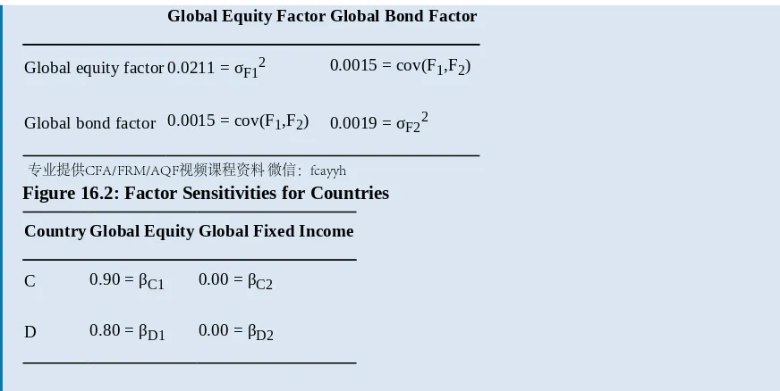
Thom Jones is a senior strategist examining equity and bond markets in countries C and D. He assigns the quantitative group to prepare a series of consistent calculations for the two markets. The group begins at Level 1 by assuming there are two factors driving the returns for all assets—a global equity factor and a global bond factor. At Level 2, this data is used to analyze each market. The data used is shown in Figure 16.1 and Figure 16.2:
Global Equity Factor Global Bond Factor
Global equity factor 0.0211 = σF12 0.0015 = cov(F1,F2)
Global bond factor 0.0015 = cov(F1,F2) 0.0019 = σF22
Figure 16.2: Factor Sensitivities for Countries
Country Global Equity Global Fixed Income
C 0.90 = βC1 0.00 = βC2
D 0.80 = βD1 0.00 = βD2
The 0.00 sensitivities to global fixed income in country markets C and D indicate both markets are equity markets. (Note that this does not mean the pairwise correlation between each market and the global bond market is zero. It means that, once the effect of the equity market is controlled for, the partial correlation of each market and the global bond factor is zero.)
Estimate the covariance between markets C and D:
Cov(C,D) = (0.90)(0.80)(0.0211) + (0)(0)(0.0019) + [(0.90)(0) + (0.00)(0.80)]0.0015 = 0.0152
Estimate the variance for market C:
(0.90)2(0.0211) + (0.00)2(0.0019) + 2(0.90)(0.00)(0.0015) = 0.0171 For market D, this is:
(0.80)2(0.0211) + (0.00)2(0.0019) + 2(0.80)(0.00)(0.0015) = 0.0135
Note that the variance of the markets will be higher than estimated because the analysis has not accounted for the variance of residual risk (σ2ε). Each market will have residual or idiosyncratic risk not explained by that market’s factor sensitivities.
Discounted Cash Flow Models
A second tool for setting capital market expectations is discounted cash flow models. These models say that the intrinsic value of an asset is the present value of future cash flows. The advantage of these models is their correct emphasis on the future cash flows of an asset and the ability to back out a required return. Their disadvantage is that they do not account for current market conditions such as supply and demand, so these models are viewed as being more suitable for long-term valuation.
Applied to equity markets, the most common application of discounted cash flow models is the Gordon growth model or constant growth model. It is most commonly used to back out the expected return on equity, resulting in the following:
where:
= expected return on stock i
Div1 = divident next period
P0 = current stock price
g = growth rate in dividends and long-term earnings
This formulation can be applied to entire markets as well. In this case, the growth rate is proxied by the nominal growth in GDP, which is the sum of the real growth rate in GDP plus the rate of inflation. The growth rate can be adjusted for any differences between the economy’s growth rate and that of the equity index. This adjustment is referred to as the excess corporate growth rate. For example, the analyst may project the U.S. real growth in GDP at 2%. If the analyst thinks that the constituents of the Wilshire 5000 index will grow at a rate 1% faster than the economy as a whole, the projected growth for the Wilshire 5000 would be 3%.
Grinold and Kroner (2002)1 take this model one step further by including a variable that adjusts for stock repurchases and changes in market valuations as represented by the price-earnings (P/E) ratio. The model states that the expected return on a stock is its dividend yield plus the inflation rate plus the real earnings growth rate minus the change in stock outstanding plus changes in the P/E ratio:
where:
= expected return on stock i; referred to as compound annual growth rate on a Level III exam
= expected divident yield
i = expected inflation g = real growth rate
ΔS = percentage change in shares outstanding (positive or negative)
The variables of the Grinold-Kroner model can be grouped into three components: the expected income return, the expected nominal growth in earnings, and the expected repricing return.
1. The expected income return is the cash flow yield for that market:
D1 / P0 is current yield as seen in the constant growth dividend discount model. It is the expected dividend expressed as a percentage of the current price. The Grinold-Kroner model goes a step further in expressing the expected current yield by considering any repurchases or new issues of stock.
PROFESSOR’S NOTE
To keep the ΔS analysis straight, just remember net stock:
Repurchase increases cash flow to investors and increases expected return. Issuance decreases cash flow to investors and decreases expected return.
The long way around to reaching these conclusions is:
Repurchase is a reduction in shares outstanding, and –ΔS, when subtracted in GK, is –(–ΔS), which becomes +ΔS and an addition to expected return. Issuance is an increase in shares outstanding, and +ΔS, when subtracted in GK, becomes –ΔS and a reduction in expected return.
2. The expected nominal earnings growth is the real growth in the stock price plus expected inflation (think of a nominal interest rate that includes the real rate plus inflation):
expected nominal earnings growth = (i + g)
3. The repricing return is captured by the expected change in the P/E ratio:
expected repricing return =
It is helpful to view the Grinold-Kroner model as the sum of the expected income return, the expected nominal growth, and the expected repricing return.
The total expected return on the stock market is 1.6% + 7.4% = 9.0%.
Estimating Fixed Income Returns
Discounted cash flow analysis of fixed income securities supports the use of YTM as an estimate of expected return. YTM is an IRR calculation and, like any IRR
calculation, it will be the realized return earned if the cash flows are reinvested at the YTM and the bond is held to maturity. For zero-coupon bonds, there are no cash flows to reinvest, though the held-to-maturity assumption still applies. Alternatively, the analyst can make other reinvestment and holding period assumptions to project expected return.
MODULE QUIZ 16.2
To best evaluate your performance, enter your quiz answers online.
1. An analyst realizes that the variance for an exchange rate tends to persist over a period of time, where high volatility is followed by more high volatility. What statistical tool would the analyst most likely use to forecast the variance of the exchange rate?
2. At the beginning of the fiscal year, Tel-Pal, Inc., stock sells for $75 per share. There are 2,000,000 shares outstanding. An analyst predicts that the annual dividend to be paid in one year will be $3 per share. The expected inflation rate is 3.5%. The firm plans to issue 40,000 new shares over the year. The price-to-earnings ratio is expected to stay the same, and nominal earnings will increase by 6.8%. Based upon these figures, what is the expected return on a share of Tel-Pal, Inc., stock in the next year?
Video covering this content is available online.
predicts the covariance will be 784. The analyst weights the historical covariance at 30% and the forecast at 70%. Calculate the shrinkage estimate of the
covariance.
MODULE 16.3: RISK PREMIUMS, FINANCIAL
EQUILIBRIUM, AND SURVEYS
An alternative to estimating expected return using YTM is a risk premium or buildup model. Risk premium approaches can be used for both fixed income and equity. The approach starts with a lower risk yield and then adds compensation for risks. A typical fixed income buildup might calculate expected return as:
RB = real risk-free rate + inflation risk premium + default risk
premium + illiquidity risk premium + maturity risk premium + tax premium The inflation premium compensates for a loss in purchasing power over time. The default risk premium compensates for possible non-payment.
The illiquidity premium compensates for holding illiquid bonds.
The maturity risk premium compensates for the greater price volatility of longer-term bonds.
The tax premium accounts for different tax treatments of some bonds.
To calculate an expected equity return, an equity risk premium would be added to the bond yield.
PROFESSOR’S NOTE
Equity buildup models vary in the starting point.
Begin with rf. The Security Market Line starts with rf and can be considered a variation of this approach.
Other models start with a long-term default free bond. Or the corporate bond yield of the issuer.
The point is to use the data provided.
Financial Equilibrium Models
The financial equilibrium approach assumes that supply and demand in global asset markets are in balance. In turn, financial models will value securities correctly. One such model is the International Capital Asset Pricing Model (ICAPM). The Singer and Terhaar approach begins with the ICAPM.
where:
= expected return on asset i
RF = risk-free rate of return
βi = sensitivity (systematic risk)of asset i returns to the global investable market
= expected return on the global investable market
Think of the global investable market as consisting of all investable assets, traditional and alternative.
We can manipulate this formula to solve for the risk premium on a debt or equity security using the following steps:
Step 1: The relationship between the covariance and correlation is:
where:
ρi,M = correlation between the returns on asset i and the global market portfolio
σi = standard deviation of the returns on asset i
σM = standard deviation of the returns on the global market portfolio
Step 2: Recall that:
where:
Cov(i,m) = covariance of asset i with the global market portfolio = variance of the returns on the global market portfolio
Step 4: Rearranging the ICAPM, we arrive at the expression for the risk premium for asset i, RPi:
The final expression states that the risk premium for an asset is equal to its correlation with the global market portfolio multiplied by the standard deviation of the asset multiplied by the Sharpe ratio for the global portfolio (in parentheses). From this formula, we forecast the risk premium and expected return for a market.
EXAMPLE: Calculating an equity risk premium and a debt risk premium
Given the following data, calculate the equity and debt risk premiums for Country X:
Expected Standard Deviation Correlation With Global Investable Market
Country X bonds 10% 0.40
Country X equities 15% 0.70
Market Sharpe ratio = 0.35
To estimate the size of the liquidity risk premium, one could estimate the multi-period Sharpe ratio for the investment over the time until it is liquid and compare it to the estimated multi-period Sharpe ratio for the market. The Sharpe ratio for the illiquid asset must be at least as high as that for the market. For example, suppose a venture capital investment has a lock-up period of five years and its multi-period Sharpe ratio is below that of the market’s. If its expected return from the ICAPM is 16%, and the return necessary to equate its Sharpe ratio to that of the market’s was 25%, then the liquidity premium would be 9%.
When markets are segmented, capital does not flow freely across borders. The opposite of segmented markets is integrated markets, where capital flows freely. Government restrictions on investing are a frequent cause of market segmentation. If markets are segmented, two assets with the same risk can have different expected returns because capital cannot flow to the higher return asset. The presence of investment barriers increases the risk premium for securities in segmented markets.
In reality, most markets are not fully segmented or integrated. For example, investors have a preference for their own country’s equity markets (the home country bias). This prevents them from fully exploiting investment opportunities overseas. Developed world equity markets have been estimated as 80% integrated, whereas emerging market equities have been estimated as 65% integrated. In the example to follow, we will adjust for partial market segmentation by estimating an equity risk premium assuming full integration and an equity risk premium assuming full segmentation, and then taking a weighted average of the two. Under the full segmentation assumption, the relevant global portfolio is the individual market so that the correlation between the market and the global portfolio in the formula is 1. In that case, the equation for the market’s risk premium reduces to:
In the following example, we will calculate the equity risk premium for the two markets, their expected returns, and the covariance between them. Before we start, recall from our discussion of factor models that the covariance between two markets given two factors is:
If there is only one factor driving returns (i.e., the global portfolio), then the equation reduces to:
Suppose an analyst is valuing two equity markets. Market A is a developed market, and Market B is an emerging market. The investor’s time horizon is five years. The other pertinent facts are:
Sharpe ratio of the global investable portfolio 0.29 Standard deviation of the global investable portfolio 9% Risk-free rate of return 5% Degree of market integration for Market A 80% Degree of market integration for Market B 65% Standard deviation of Market A 17% Standard deviation of Market B 28% Correlation of Market A with global investable portfolio 0.82 Correlation of Market B with global investable portfolio 0.63 Estimated illiquidity premium for A 0.0% Estimated illiquidity premium for B 2.3%
Calculate the assets’ expected returns, betas, and covariance.
Answer:
First, we calculate the equity risk premium for both markets assuming full integration. Note that for the emerging market, the illiquidity risk premium is included:
ERPi = ρi,Mσi(market Sharpe ratio) ERPA = (0.82)(0.17)(0.29) = 4.04%
ERPB = (0.63)(0.28)(0.29) + 0.0230 = 7.42%
Next, we calculate the equity risk premium for both markets assuming full segmentation: ERPi = σi(market Sharpe ratio)
ERPA = (0.17)(0.29) = 4.93%
ERPB = (0.28)(0.29) + 0.0230 = 10.42%
Note that when we calculate the risk premium under full segmentation, we use the local market as the reference market instead of the global market, so the correlation between the local market and itself is 1.0.
We then weight the integrated and segmented risk premiums by the degree of integration and segmentation in each market to arrive at the weighted average equity risk premium.
ERPi = (degree of integration of i)(ERP assuming full integration) + (degree of segmentation of i)(ERP assuming full segmentation)
ERPA = (0.80)(0.0404) + (1 − 0.80)(0.0493) = 4.22% ERPB = (0.65)(0.0742) + (1 − 0.65)(0.1042) = 8.47% The expected return in each market figures in the risk-free rate:
Video covering this content is available online.
Lastly, we calculate the covariance of the two equity markets:
PROFESSOR’S NOTE
Theoretically, a fully segmented market’s Sharpe ratio would be independent of the world market Sharpe ratio. However, the CFA text makes the simplifying assumption to use the world market Sharpe ratio in both the segmented and integrated calculations. This is a reasonable assumption as we are valuing partially integrated/segmented markets. There is no reason to analyze the fully segmented market as outsiders cannot, by definition, invest in such markets.
THE USE OF SURVEYS AND JUDGMENT FOR CAPITAL
MARKET EXPECTATIONS
LOS 16.d: Explain the use of survey and panel methods and judgment in setting capital market expectations.
CFA® Program Curriculum, Volume 3, page 48
Capital market expectations can also be formed using surveys. In this method, a poll is taken of market participants, such as economists and analysts, as to what their
expectations are regarding the economy or capital market. If the group polled is fairly constant over time, this method is referred to as a panel method. For example, the U.S. Federal Reserve Bank of Philadelphia conducts an ongoing survey regarding the U.S. consumer price index, GDP, and so forth.2
Judgment can also be applied to project capital market expectations. Although quantitative models provide objective numerical forecasts, there are times when an analyst must adjust those expectations using their experience and insight to improve upon those forecasts.
MODULE 16.4: THE BUSINESS CYCLE
LOS 16.e: Discuss the inventory and business cycles and the effects that consumer and business spending and monetary and fiscal policy have on the business cycle.
CFA® Program Curriculum, Volume 3, page 50
Understanding the business cycle can help the analyst identify inflection points (i.e., when the economy changes direction), where the risk and the opportunities for higher return may be heightened. To identify inflection points, the analyst should understand what is driving the current economy and what may cause the end of the current
economy.
In general, economic growth can be partitioned into two components: (1) cyclical and (2) trend-growth components. The former is more short-term whereas the latter is more relevant for determining long-term return expectations. We will discuss the cyclical component first.
Within cyclical analysis, there are two components: (1) the inventory cycle and (2) the business cycle. The former typically lasts two to four years whereas the latter has a typical duration of nine to eleven years. These cycles vary in duration and are hard to predict because wars and other events can disrupt them.
Changes in economic activity delineate cyclical activity. The measures of economic activity are GDP, the output gap, and a recession. GDP is usually measured in real terms because true economic growth should be adjusted for inflationary components. The output gap is the difference between GDP based on a long-term trend line (i.e., potential GDP) and the current level of GDP. When the trend line is higher than the current GDP, the economy has slowed and inflationary pressures have weakened. When it is lower, economic activity is strong, as are inflationary pressures. This relationship is used by policy makers to form expectations regarding the appropriate level of growth and inflation. The relationship is affected by changes in technology and demographics. The third measure of economic activity, a recession, is defined as decreases (i.e., negative growth) in GDP over two consecutive quarters.
The inventory cycle is thought to be 2 to 4 years in length. It is often measured using the inventory to sales ratio. The measure increases when businesses gain confidence in the future of the economy and add to their inventories in anticipation of increasing demand for their output. As a result, employment increases with subsequent increases in economic growth. This continues until some precipitating factor, such as a tightening in the growth of the money supply, intervenes. At this point, inventories decrease and employment declines, which causes economic growth to slow.
When the inventory measure has peaked in an economy, as in the United States in 2000, subsequent periods exhibit slow growth as businesses sell out of their inventory. When it bottoms out, as in 2004, subsequent periods have higher growth as businesses restock their inventory. The long-term trend in this measure has been downward due to more effective inventory management techniques such as just-in-time inventory management. The longer-term business cycle is thought to be 9 to 11 years in length. It is
characterized by five phases: (1) the initial recovery, (2) early upswing, (3) late upswing, (4) slowdown, and (5) recession. We discuss the business cycle in greater detail later when we examine its effect on asset returns.
LOS 16.f: Discuss the effects that the phases of the business cycle have on short-term/long-term capital market returns.
For the Exam: Have a working knowledge of, and be able to explain, the general relationships between interest rates, inflation, stock and bond prices, inventory levels, et cetera, as you progress over the business cycle. For example, as the peak of the cycle approaches, everything is humming along. Confidence and employment are high, but inflation is starting to have an impact on markets. As inflation increases, bond yields increase and both bond and stock prices start to fall.
The Business Cycle and Asset Returns
The relationship between the business cycle and assets returns is well-documented. Assets with higher returns during business cycle lows (e.g., bonds and defensive stocks) should be favored by investors because the returns supplement their income during recessionary periods. These assets should have lower risk premiums. Assets with lower returns during recessions should have higher risk premiums. Understanding the
relationship between an asset’s return and the business cycle can help the analyst provide better valuations.
As mentioned before, inflation varies over the business cycle, which has five phases: (1) initial recovery, (2) early expansion, (3) late expansion, (4) slowdown, and (5)
recession. Inflation rises in the latter stages of an expansion and falls during a recession and the initial recovery. The phases have the following characteristics:
Initial Recovery
Duration of a few months. Business confidence is rising.
Government stimulation is provided by low interest rates and/or budget deficits. Falling inflation.
Large output gap
Low or falling short-term interest rates. Bond yields are bottoming out.
Rising stock prices.
Cyclical, riskier assets such as small-cap stocks and high yield bonds do well.
Early Upswing
Duration of a year to several years. Increasing growth with low inflation. Increasing confidence.
Increasing inventories.
Late Upswing
Confidence and employment are high.
Output gap eliminated and economy at risk of overheating. Inflation increases.
Central bank limits the growth of the money supply. Rising short-term interest rates.
Rising bond yields.
Rising/peaking stock prices with increased risk and volatility.
Slowdown
Duration of a few months to a year or longer. Declining confidence.
Inflation is still rising. Falling inventory levels.
Short-term interest rates are at a peak.
Bond yields have peaked and may be falling, resulting in rising bond prices. Yield curve may invert.
Falling stock prices.
Recession
Duration of six months to a year. Large declines in inventory. Declining confidence and profits.
Increase in unemployment and bankruptcies. Inflation tops out.
Falling short-term interest rates. Falling bond yields, rising prices.
Stock prices increase during the latter stages anticipating the end of the recession.
Inflation
Inflation means generally rising prices. For example, if the CPI index increases from 100 to 105, inflation is 5%. Inflation typically accelerates late in the business cycle (near the peak).
Inflation typically decelerates as the economy approaches and enters recession. Deflation means generally falling prices. For example, if the CPI index declines from 108 to 106, the rate of inflation is approximately –2%. Deflation is a severe threat to economic activity:
It encourages default on debt obligations. Consider a homeowner who has a home worth $100,000 and a mortgage of $95,000; the homeowner’s equity is only $5,000. A decline of more than 5% in home prices leads to negative equity and can trigger panic sales (further depressing prices), defaulting on the loan, or both. With negative inflation, interest rates decline to near zero and this limits the ability of central banks to lower interest rates and stimulate the economy.
Following the financial crisis of 2007–09 and the resulting very low interest rates, several central banks tried a new monetary policy of quantitative easing (QE) to stimulate the economies of their countries. Traditionally, central banks have used open markets to increase the money supply and lower short-term interest rates on a temporary basis by buying high quality fixed-income instruments. QE was different in that it was larger in scale, the purchases included other security types such as mortgage-backed securities and corporate bonds, and the intent was a long-term increase in bank reserves, not temporary.
INFLATION AND ASSET RETURNS
LOS 16.g: Explain the relationship of inflation to the business cycle and the implications of inflation for cash, bonds, equity, and real estate returns.
CFA® Program Curriculum, Volume 3, page 58
The
ST rates low or declining LT rates bottoming and bond prices peaking
Stock prices increasing
Early
upswing Low inflation and goodeconomic growth Becoming lessstimulative
ST rates increasing LT rates bottoming or increasing with bond prices beginning to decline
Stock prices increasing
Late
upswing Inflation rate increasing Becomingrestrictive
ST and LT rates increasing with bond prices declining
Stock prices peaking and volatile
Slowdown Inflation continues toaccelerate Becoming lessrestrictive
ST and LT rates peaking and then declining with bond prices starting to increase
Recession Real economic activity
declining and inflation peaking Easing ST and LT rates declining with bond pricesincreasing Stock prices begin to increase later in the recession
Inflation and Relative Attractiveness of Asset Classes
Inflation at or below
expectations Cash Equivalents (CE) and Bonds: Neutral with stable or declining yields Equity: Positive with predictable economic growth Real Estate (RE): Neutral with typical rates of return
Inflation above
expectations CE: Positive with increasing yields
Bonds: Negative as rates increase and prices decline
Equity: Negative, though some companies may be able to pass through inflation and do well
RE: Positive as real asset values increase with inflation
Deflation
CE: Negative with approximately 0% interest rates
Bonds: Positive as the fixed future cash flows have greater purchasing power (assuming no default on the bonds)
Equity: Negative as economic activity and business declines RE: Negative as property values generally decline
PROFESSOR’S NOTE
Please note that these are generalizations that will not hold in every case. They are a good starting point for a forecaster taking a macro approach. Even if the generalizations always held, it is not easy to determine when a business cycle phase starts, how long it will last, or when it ends.
Consumer and Business Spending
As a percentage of GDP, consumer spending is much larger than business spending. Consumer spending is usually gauged through the use of store sales data, retail sales, and consumer consumption data. The data has a seasonal pattern, with sales increasing near holidays. In turn, the primary driver of consumer spending is consumer after-tax income, which in the United States is gauged using non-farm payroll data and new unemployment claims. Employment data is important to markets because it is usually quite timely.
Given that spending is income net of savings, savings data are also important for
the business cycle) and reversed. At this point, consumers begin saving more and more until the economy “turns the corner,” and the cycle starts over.
Business spending is more volatile than consumer spending. Spending by businesses on inventory and investments is quite volatile over the business cycle. As mentioned before, the peak of inventory spending is often a bearish signal for the economy. It may indicate that businesses have overspent relative to the amount they are selling. This portends a slowdown in business spending and economic growth.
MODULE QUIZ 16.3, 16.4
To best evaluate your performance, enter your quiz answers online.
1. Suppose an analyst is valuing two markets, A and B. What is the equity risk premium for the two markets, their expected returns, and the covariance between them, given the following?
Sharpe ratio of the global portfolio 0.29
Standard deviation of the global portfolio 8.0%
Risk-free rate of return 4.5%
Degree of market integration for Market A 80%
Degree of market integration for Market B 65%
Standard deviation of Market A 18%
Standard deviation of Market B 26%
Correlation of Market A with global portfolio 0.87
Correlation of Market B with global portfolio 0.63
Estimated illiquidity premium for Market A 0.0%
Estimated illiquidity premium for Market B 2.4%