Tensor Calculus
and
Continuum Mechanics
by J.H. Heinbockel
Department of Mathematics and Statistics
This is an introductory text which presents fundamental concepts from the subject
areas of tensor calculus, differential geometry and continuum mechanics. The material
presented is suitable for a two semester course in applied mathematics and is flexible
enough to be presented to either upper level undergraduate or beginning graduate students
majoring in applied mathematics, engineering or physics. The presentation assumes the
students have some knowledge from the areas of matrix theory, linear algebra and advanced
calculus. Each section includes many illustrative worked examples. At the end of each
section there is a large collection of exercises which range in difficulty. Many new ideas
are presented in the exercises and so the students should be encouraged to read all the
exercises.
The purpose of preparing these notes is to condense into an introductory text the basic
definitions and techniques arising in tensor calculus, differential geometry and continuum
mechanics. In particular, the material is presented to (i) develop a physical understanding
of the mathematical concepts associated with tensor calculus and (ii) develop the basic
equations of tensor calculus, differential geometry and continuum mechanics which arise
in engineering applications. From these basic equations one can go on to develop more
sophisticated models of applied mathematics. The material is presented in an informal
manner and uses mathematics which minimizes excessive formalism.
The material has been divided into two parts. The first part deals with an
introduc-tion to tensor calculus and differential geometry which covers such things as the indicial
notation, tensor algebra, covariant differentiation, dual tensors, bilinear and multilinear
forms, special tensors, the Riemann Christoffel tensor, space curves, surface curves,
cur-vature and fundamental quadratic forms. The second part emphasizes the application of
tensor algebra and calculus to a wide variety of applied areas from engineering and physics.
The selected applications are from the areas of dynamics, elasticity, fluids and
electromag-netic theory. The continuum mechanics portion focuses on an introduction of the basic
concepts from linear elasticity and fluids. The Appendix A contains units of measurements
from the Syst`eme International d’Unit`es along with some selected physical constants. The
Appendix B contains a listing of Christoffel symbols of the second kind associated with
various coordinate systems. The Appendix C is a summary of useful vector identities.
AND
CONTINUUM MECHANICS
PART 1: INTRODUCTION TO TENSOR CALCULUS
§
1.1 INDEX NOTATION
. . . .
1
Exercise 1.1
. . . .
28
§
1.2 TENSOR CONCEPTS AND TRANSFORMATIONS
. . . .
35
Exercise 1.2
. . . .
54
§
1.3 SPECIAL TENSORS
. . . .
65
Exercise 1.3
. . . .
101
§
1.4 DERIVATIVE OF A TENSOR
. . . .
108
Exercise 1.4
. . . .
123
§
1.5 DIFFERENTIAL GEOMETRY AND RELATIVITY
. . . .
129
Exercise 1.5
. . . .
162
PART 2: INTRODUCTION TO CONTINUUM MECHANICS
§
2.1 TENSOR NOTATION FOR VECTOR QUANTITIES
. . . .
171
Exercise 2.1
. . . .
182
§
2.2 DYNAMICS
. . . .
187
Exercise 2.2
. . . .
206
§
2.3 BASIC EQUATIONS OF CONTINUUM MECHANICS
. . .
211
Exercise 2.3
. . . .
238
§
2.4 CONTINUUM MECHANICS (SOLIDS)
. . . .
243
Exercise 2.4
. . . .
272
§
2.5 CONTINUUM MECHANICS (FLUIDS)
. . . .
282
Exercise 2.5
. . . .
317
§
2.6 ELECTRIC AND MAGNETIC FIELDS
. . . .
325
Exercise 2.6
. . . .
347
BIBLIOGRAPHY
. . . .
352
APPENDIX A
UNITS OF MEASUREMENT
. . . .
353
APPENDIX B
CHRISTOFFEL SYMBOLS OF SECOND KIND
355
APPENDIX C
VECTOR IDENTITIES
. . . .
362
PART 1: INTRODUCTION TO TENSOR CALCULUS
A scalar field describes a one-to-one correspondence between a single scalar number and a point. An n-dimensional vector field is described by a one-to-one correspondence between n-numbers and a point. Let us generalize these concepts by assigning n-squared numbers to a single point orn-cubed numbers to a single point. When these numbers obey certain transformation laws they become examples of tensor fields. In general, scalar fields are referred to as tensor fields of rank or order zero whereas vector fields are called tensor fields of rank or order one.
Closely associated with tensor calculus is the indicial or index notation. In section 1 the indicial notation is defined and illustrated. We also define and investigate scalar, vector and tensor fields when they are subjected to various coordinate transformations. It turns out that tensors have certain properties which are independent of the coordinate system used to describe the tensor. Because of these useful properties, we can use tensors to represent various fundamental laws occurring in physics, engineering, science and mathematics. These representations are extremely useful as they are independent of the coordinate systems considered.
§1.1 INDEX NOTATION
Two vectorsA andB can be expressed in the component form
A=A1e1+A2e2+A3e3 and B =B1e1+B2e2+B3e3,
where e1, e2 and e3 are orthogonal unit basis vectors. Often when no confusion arises, the vectorsA and
B are expressed for brevity sake as number triples. For example, we can write
A= (A1, A2, A3) and B = (B1, B2, B3)
where it is understood that only the components of the vectorsA andB are given. The unit vectors would be represented
e1= (1,0,0), e2= (0,1,0), e3= (0,0,1).
A still shorter notation, depicting the vectorsAandB is the index or indicial notation. In the index notation, the quantities
Ai, i= 1,2,3 and Bp, p= 1,2,3
represent the components of the vectorsAandB. This notation focuses attention only on the components of the vectors and employs a dummy subscript whose range over the integers is specified. The symbolAirefers
to all of the components of the vectorA simultaneously. The dummy subscriptican have any of the integer values 1,2 or 3.For i= 1 we focus attention on the A1 component of the vector A. Setting i= 2 focuses
attention on the second component A2 of the vectorA and similarly wheni= 3 we can focus attention on
the third component ofA. The subscriptiis a dummy subscript and may be replaced by another letter, say
It is also convenient at this time to mention that higher dimensional vectors may be defined as ordered
n−tuples. For example, the vector
X = (X1, X2, . . . , XN)
with components Xi, i= 1,2, . . . , N is called aN−dimensional vector. Another notation used to represent
this vector is
X=X1e1+X2e2+· · ·+XNeN
where
e1, e2, . . . ,eN
are linearly independent unit base vectors. Note that many of the operations that occur in the use of the index notation apply not only for three dimensional vectors, but also forN−dimensional vectors.
In future sections it is necessary to define quantities which can be represented by a letter with subscripts or superscripts attached. Such quantities are referred to as systems. When these quantities obey certain transformation laws they are referred to as tensor systems. For example, quantities like
Ak
ij eijk δij δji Ai Bj aij.
The subscripts or superscripts are referred to as indices or suffixes. When such quantities arise, the indices must conform to the following rules:
1. They are lower case Latin or Greek letters.
2. The letters at the end of the alphabet (u, v, w, x, y, z) are never employed as indices.
The number of subscripts and superscripts determines the order of the system. A system with one index is a first order system. A system with two indices is called a second order system. In general, a system with
N indices is called aNth order system. A system with no indices is called a scalar or zeroth order system. The type of system depends upon the number of subscripts or superscripts occurring in an expression. For example, Aijk and Bstm, (all indices range 1 to N), are of the same type because they have the same
number of subscripts and superscripts. In contrast, the systems Aijk and Cpmn are not of the same type
because one system has two superscripts and the other system has only one superscript. For certain systems the number of subscripts and superscripts is important. In other systems it is not of importance. The meaning and importance attached to sub- and superscripts will be addressed later in this section.
In the use of superscripts one must not confuse “powers ”of a quantity with the superscripts. For example, if we replace the independent variables (x, y, z) by the symbols (x1, x2, x3),then we are letting
y = x2 where x2 is a variable and not x raised to a power. Similarly, the substitution z = x3 is the replacement of z by the variablex3 and this should not be confused with xraised to a power. In order to write a superscript quantity to a power, use parentheses. For example, (x2)3 is the variable x2 cubed. One
of the reasons for introducing the superscript variables is that many equations of mathematics and physics can be made to take on a concise and compact form.
the Kronecker delta symbol δij, defined by δij = 1 ifi=j and δij = 0 for i=j, withi, j ranging over the
values 1,2,3, represents the 9 quantities
δ11= 1
δ21= 0
δ31= 0
δ12= 0
δ22= 1
δ32= 0
δ13= 0
δ23= 0
δ33= 1.
The symbolδij refers to all of the components of the system simultaneously. As another example, consider
the equation
em· en=δmn m, n= 1,2,3 (1.1.1)
the subscriptsm, noccur unrepeated on the left side of the equation and hence must also occur on the right hand side of the equation. These indices are called “free ”indices and can take on any of the values 1,2 or 3 as specified by the range. Since there are three choices for the value form and three choices for a value of
nwe find that equation (1.1.1) represents nine equations simultaneously. These nine equations are
e1· e1= 1
e2· e1= 0
e3· e1= 0
e1·e2= 0 e2·e2= 1 e3·e2= 0
e1· e3= 0
e2· e3= 0
e3· e3= 1. Symmetric and Skew-Symmetric Systems
A system defined by subscripts and superscripts ranging over a set of values is said to be symmetric in two of its indices if the components are unchanged when the indices are interchanged. For example, the third order systemTijk is symmetric in the indicesiand kif
Tijk =Tkji for all values ofi, j andk.
A system defined by subscripts and superscripts is said to be skew-symmetric in two of its indices if the components change sign when the indices are interchanged. For example, the fourth order system Tijkl is
skew-symmetric in the indicesiandl if
Tijkl=−Tljki for all values ofijk andl.
As another example, consider the third order system aprs, p, r, s = 1,2,3 which is completely
skew-symmetric in all of its indices. We would then have
aprs=−apsr=aspr =−asrp=arsp=−arps.
It is left as an exercise to show this completely skew- symmetric systems has 27 elements, 21 of which are zero. The 6 nonzero elements are all related to one another thru the above equations when (p, r, s) = (1,2,3).
Summation Convention
The summation convention states that whenever there arises an expression where there is an index which occurs twice on the same side of any equation, or term within an equation, it is understood to represent a summation on these repeated indices. The summation being over the integer values specified by the range. A repeated index is called a summation index, while an unrepeated index is called a free index. The summation convention requires that one must never allow a summation index to appear more than twice in any given expression. Because of this rule it is sometimes necessary to replace one dummy summation symbol by some other dummy symbol in order to avoid having three or more indices occurring on the same side of the equation. The index notation is a very powerful notation and can be used to concisely represent many complex equations. For the remainder of this section there is presented additional definitions and examples to illustrated the power of the indicial notation. This notation is then employed to define tensor components and associated operations with tensors.
EXAMPLE 1.1-1 The two equations
y1=a11x1+a12x2
y2=a21x1+a22x2
can be represented as one equation by introducing a dummy index, sayk,and expressing the above equations as
yk=ak1x1+ak2x2, k= 1,2.
The range convention states that k is free to have any one of the values 1 or 2, (k is a free index). This equation can now be written in the form
yk =
2
i=1
akixi=ak1x1+ak2x2
whereiis the dummy summation index. When the summation sign is removed and the summation convention is adopted we have
yk =akixi i, k= 1,2.
Since the subscript irepeats itself, the summation convention requires that a summation be performed by letting the summation subscript take on the values specified by the range and then summing the results. The index k which appears only once on the left and only once on the right hand side of the equation is called a free index. It should be noted that bothkandiare dummy subscripts and can be replaced by other letters. For example, we can write
yn=anmxm n, m= 1,2
where mis the summation index andnis the free index. Summing onmproduces
yn=an1x1+an2x2
EXAMPLE 1.1-2. For yi =aijxj, i, j = 1,2,3 and xi = bijzj, i, j = 1,2,3 solve for the y variables in
terms of the zvariables.
Solution: In matrix form the given equations can be expressed:
Now solve for the yvariables in terms of thez variables and obtain
The index notation employs indices that are dummy indices and so we can write
yn=anmxm, n, m= 1,2,3 and xm=bmjzj, m, j= 1,2,3.
Here we have purposely changed the indices so that when we substitute forxm, from one equation into the
other, a summation index does not repeat itself more than twice. Substituting we find the indicial form of the above matrix equation as
yn=anmbmjzj, m, n, j= 1,2,3
where n is the free index and m, j are the dummy summation indices. It is left as an exercise to expand both the matrix equation and the indicial equation and verify that they are different ways of representing the same thing.
EXAMPLE 1.1-3. The dot product of two vectorsAq, q= 1,2,3 andBj, j = 1,2,3 can be represented
with the index notation by the product AiBi = ABcosθ i = 1,2,3, A = |A|, B = |B|. Since the
subscript i is repeated it is understood to represent a summation index. Summing on i over the range specified, there results
A1B1+A2B2+A3B3=ABcosθ.
Observe that the index notation employs dummy indices. At times these indices are altered in order to conform to the above summation rules, without attention being brought to the change. As in this example, the indicesqandjare dummy indices and can be changed to other letters if one desires. Also, in the future, if the range of the indices is not stated it is assumed that the range is over the integer values 1,2 and 3.
Addition, Multiplication and Contraction
The algebraic operation of addition or subtraction applies to systems of the same type and order. That is we can add or subtract like components in systems. For example, the sum of Aijk and Bjki is again a
system of the same type and is denoted byCjki =Aijk+Bjki ,where like components are added.
The product of two systems is obtained by multiplying each component of the first system with each component of the second system. Such a product is called an outer product. The order of the resulting product system is the sum of the orders of the two systems involved in forming the product. For example, if Ai
j is a second order system and Bmnl is a third order system, with all indices having the range 1 to N,
then the product system is fifth order and is denotedCjimnl=AijBmnl. The product system representsN5
terms constructed from all possible products of the components fromAij with the components fromBmnl.
The operation of contraction occurs when a lower index is set equal to an upper index and the summation convention is invoked. For example, if we have a fifth order system Cjimnl and we set i=j and sum, then
we form the system
Cmnl=Cjjmnl =C11mnl+C22mnl+· · ·+CNN mnl.
Here the symbol Cmnl is used to represent the third order system that results when the contraction is
performed. Whenever a contraction is performed, the resulting system is always of order 2 less than the original system. Under certain special conditions it is permissible to perform a contraction on two lower case indices. These special conditions will be considered later in the section.
The above operations will be more formally defined after we have explained what tensors are.
The e-permutation symbol and Kronecker delta
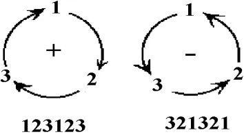
EXAMPLE 1.1-4. The total number of possible ways of arranging the digits 1 2 3 is six. We have three choices for the first digit. Having chosen the first digit, there are only two choices left for the second digit. Hence the remaining number is for the last digit. The product (3)(2)(1) = 3! = 6 is the number of permutations of the digits 1, 2 and 3. These six permutations are
1 2 3 even permutation 1 3 2 odd permutation 3 1 2 even permutation 3 2 1 odd permutation 2 3 1 even permutation 2 1 3 odd permutation.
Here a permutation of 1 2 3 is called even or odd depending upon whether there is an even or odd number of transpositions of the digits. A mnemonic device to remember the even and odd permutations of 123 is illustrated in the figure 1.1-1. Note that even permutations of 123 are obtained by selecting any three consecutive numbers from the sequence 123123 and the odd permutations result by selecting any three consecutive numbers from the sequence 321321.
Figure 1.1-1. Permutations of 123.
In general, the number of permutations ofnthings takenmat a time is given by the relation
P(n, m) =n(n−1)(n−2)· · ·(n−m+ 1).
By selecting a subset ofm objects from a collection ofn objects,m≤n, without regard to the ordering is called a combination of nobjects takenm at a time. For example, combinations of 3 numbers taken from the set{1,2,3,4}are (123),(124),(134),(234). Note that ordering of a combination is not considered. That is, the permutations (123),(132),(231),(213),(312),(321) are considered equal. In general, the number of combinations ofnobjects takenmat a time is given byC(n, m) =n
m
= n!
m!(n−m)! where
n m
are the binomial coefficients which occur in the expansion
(a+b)n=
n
m=0 n
m
The definition of permutations can be used to define the e-permutation symbol.
Definition: (e-Permutation symbol or alternating tensor)
The e-permutation symbol is defined
eijk...l=eijk...l=
1 ifijk . . . l is an even permutation of the integers 123. . . n
−1 ifijk . . . l is an odd permutation of the integers 123. . . n
0 in all other cases
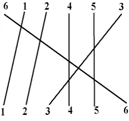
EXAMPLE 1.1-5. Finde612453.
Solution: To determine whether 612453 is an even or odd permutation of 123456 we write down the given numbers and below them we write the integers 1 through 6. Like numbers are then connected by a line and we obtain figure 1.1-2.
Figure 1.1-2. Permutations of 123456.
In figure 1.1-2, there are seven intersections of the lines connecting like numbers. The number of intersections is an odd number and shows that an odd number of transpositions must be performed. These results imply e612453=−1.
Another definition used quite frequently in the representation of mathematical and engineering quantities is the Kronecker delta which we now define in terms of both subscripts and superscripts.
Definition: (Kronecker delta) The Kronecker delta is defined:
δij =δji =
1 ifiequalsj
EXAMPLE 1.1-6. Some examples of thee−permutation symbol and Kronecker delta are:
e123=e123= +1
e213=e213=−1
e112=e112= 0
δ11= 1
δ1 2= 0
δ31= 0
δ12= 0
δ22= 1
δ32= 0.
EXAMPLE 1.1-7. When an index of the Kronecker deltaδij is involved in the summation convention,
the effect is that of replacing one index with a different index. For example, letaijdenote the elements of an
N×N matrix. Hereiandj are allowed to range over the integer values 1,2, . . . , N.Consider the product
aijδik
where the range ofi, j, k is 1,2, . . . , N.The indexiis repeated and therefore it is understood to represent a summation over the range. The index iis called a summation index. The other indicesj andk are free indices. They are free to be assigned any values from the range of the indices. They are not involved in any summations and their values, whatever you choose to assign them, are fixed. Let us assign a value ofj and
k to the values ofj andk. The underscore is to remind you that these values forj andkare fixed and not to be summed. When we perform the summation over the summation indexiwe assign values toifrom the range and then sum over these values. Performing the indicated summation we obtain
aijδik =a1jδ1k+a2jδ2k+· · ·+akjδkk+· · ·+aN jδN k.
In this summation the Kronecker delta is zero everywhere the subscripts are different and equals one where the subscripts are the same. There is only one term in this summation which is nonzero. It is that term where the summation index iwas equal to the fixed valuekThis gives the result
akjδkk=akj
where the underscore is to remind you that the quantities have fixed values and are not to be summed. Dropping the underscores we write
aijδik =akj
Here we have substituted the index ibykand so when the Kronecker delta is used in a summation process it is known as a substitution operator. This substitution property of the Kronecker delta can be used to simplify a variety of expressions involving the index notation. Some examples are:
Bijδjs=Bis
δjkδkm=δjm
eijkδimδjnδkp=emnp.
Some texts adopt the notation that if indices are capital letters, then no summation is to be performed. For example,
as δKK represents a single term because of the capital letters. Another notation which is used to denote no
summation of the indices is to put parenthesis about the indices which are not to be summed. For example,
a(k)jδ(k)(k)=akj,
since δ(k)(k) represents a single term and the parentheses indicate that no summation is to be performed.
At any time we may employ either the underscore notation, the capital letter notation or the parenthesis notation to denote that no summation of the indices is to be performed. To avoid confusion altogether, one can write out parenthetical expressions such as “(no summation onk)”.
EXAMPLE 1.1-8. In the Kronecker delta symbolδi
j we setj equal toiand perform a summation. This
operation is called a contraction. There results δi
i, which is to be summed over the range of the index i.
Utilizing the range 1,2, . . . , N we have
δii=δ11+δ22+· · ·+δNN
δii= 1 + 1 +· · ·+ 1
δi i=N.
In three dimension we haveδij, i, j= 1,2,3 and
δk
k =δ11+δ22+δ33= 3.
In certain circumstances the Kronecker delta can be written with only subscripts. For example,
δij, i, j = 1,2,3. We shall find that these circumstances allow us to perform a contraction on the lower
indices so thatδii= 3.
EXAMPLE 1.1-9. The determinant of a matrixA= (aij) can be represented in the indicial notation.
Employing the e-permutation symbol the determinant of anN×N matrix is expressed
|A|=eij...ka1ia2j· · ·aN k
where eij...kis anNth order system. In the special case of a 2×2 matrix we write |A|=eija1ia2j
where the summation is over the range 1,2 and the e-permutation symbol is of order 2. In the special case of a 3×3 matrix we have
|A|=
a11 a12 a13
a21 a22 a23
a31 a32 a33
=eijkai1aj2ak3=eijka1ia2ja3k
where i, j, k are the summation indices and the summation is over the range 1,2,3. Here eijk denotes the
more general results. Consider (p, q, r) as some permutation of the integers (1,2,3), and observe that the determinant can be expressed
∆ =
ap1 ap2 ap3
aq1 aq2 aq3
ar1 ar2 ar3
=eijkapiaqjark.
If (p, q, r) is an even permutation of (1,2,3) then ∆ =|A|
If (p, q, r) is an odd permutation of (1,2,3) then ∆ =−|A|
If (p, q, r) is not a permutation of (1,2,3) then ∆ = 0.
We can then write
eijkapiaqjark=epqr|A|.
Each of the above results can be verified by performing the indicated summations. A more formal proof of the above result is given in EXAMPLE 1.1-25, later in this section.
EXAMPLE 1.1-10. The expression eijkBijCi is meaningless since the index irepeats itself more than
twice and the summation convention does not allow this. If you really did want to sum over an index which occurs more than twice, then one must use a summation sign. For example the above expression would be written
n
i=1
eijkBijCi.
EXAMPLE 1.1-11.
The cross product of the unit vectors e1, e2, e3can be represented in the index notation by
ei× ej=
ek if (i, j, k) is an even permutation of (1,2,3) −ek if (i, j, k) is an odd permutation of (1,2,3)
0 in all other cases
This result can be written in the form ei×ej=ekijek.This later result can be verified by summing on the
index kand writing out all 9 possible combinations foriandj.
EXAMPLE 1.1-12. Given the vectorsAp, p= 1,2,3 and Bp, p= 1,2,3 the cross product of these two
vectors is a vectorCp, p= 1,2,3 with components
Ci=eijkAjBk, i, j, k= 1,2,3. (1.1.2)
The quantitiesCi represent the components of the cross product vector
C=A×B =C1e1+C2e2+C3e3.
The equation (1.1.2), which defines the components of C, is to be summed over each of the indices which repeats itself. We have summing on the indexk
We next sum on the indexj which repeats itself in each term of equation (1.1.3). This gives
Ci=ei11A1B1+ei21A2B1+ei31A3B1
+ei12A1B2+ei22A2B2+ei32A3B2
+ei13A1B3+ei23A2B3+ei33A3B3.
(1.1.4) Now we are left with ibeing a free index which can have any of the values of 1,2 or 3. Lettingi= 1,then letting i= 2,and finally lettingi= 3 produces the cross product components
C1=A2B3−A3B2
C2=A3B1−A1B3
C3=A1B2−A2B1.
The cross product can also be expressed in the form A ×B =eijkAjBkei. This result can be verified by
summing over the indicesi,jand k.
EXAMPLE 1.1-13. Show
eijk =−eikj=ejki for i, j, k= 1,2,3
Solution: The array i k j represents an odd number of transpositions of the indices i j k and to each transposition there is a sign change of the e-permutation symbol. Similarly, j k iis an even transposition of i j k and so there is no sign change of the e-permutation symbol. The above holds regardless of the numerical values assigned to the indicesi, j, k.
The e-δ Identity
An identity relating the e-permutation symbol and the Kronecker delta, which is useful in the simpli-fication of tensor expressions, is the e-δ identity. This identity can be expressed in different forms. The subscript form for this identity is
eijkeimn=δjmδkn−δjnδkm, i, j, k, m, n= 1,2,3
where iis the summation index and j, k, m, nare free indices. A device used to remember the positions of the subscripts is given in the figure 1.1-3.
The subscripts on the four Kronecker delta’s on the right-hand side of the e-δ identity then are read (first)(second)-(outer)(inner).
Figure 1.1-3. Mnemonic device for position of subscripts.
Another form of this identity employs both subscripts and superscripts and has the form
eijkeimn=δmjδnk−δnjδkm. (1.1.5)
One way of proving this identity is to observe the equation (1.1.5) has the free indicesj, k, m, n.Each of these indices can have any of the values of 1,2 or 3. There are 3 choices we can assign to each ofj, k, m
or nand this gives a total of 34= 81 possible equations represented by the identity from equation (1.1.5).
By writing out all 81 of these equations we can verify that the identity is true for all possible combinations that can be assigned to the free indices.
An alternate proof of the e−δidentity is to consider the determinant
By performing a permutation of the rows of this matrix we can use the permutation symbol and write
By performing a permutation of the columns, we can write
Now perform a contraction on the indicesi andrto obtain
Generalized Kronecker delta
The generalized Kronecker delta is defined by the (n×n) determinant
δmn...pij...k =
δi
m δin · · · δpi
δj
m δjn · · · δpj
..
. ... . .. ...
δk
m δkn · · · δpk
.
For example, in three dimensions we can write
δijk mnp=
δi
m δni δpi
δj
m δnj δpj
δk
m δnk δkp
=eijke mnp.
Performing a contraction on the indicesk andpwe obtain the fourth order system
δmnrs =δrspmnp=erspemnp=eprsepmn=δrmδsn−δrnδms.
As an exercise one can verify that the definition of the e-permutation symbol can also be defined in terms of the generalized Kronecker delta as
ej1j2j3···jN =δ
1 2 3···N j1j2j3···jN.
Additional definitions and results employing the generalized Kronecker delta are found in the exercises. In section 1.3 we shall show that the Kronecker delta and epsilon permutation symbol are numerical tensors which have fixed components in every coordinate system.
Additional Applications of the Indicial Notation
The indicial notation, together with thee−δidentity, can be used to prove various vector identities.
EXAMPLE 1.1-14. Show, using the index notation, thatA×B =−B ×A
Solution: Let
C=A×B =C1e1+C2e2+C3e3=Ciei and let
D=B ×A=D1e1+D2e2+D3e3=Diei.
We have shown that the components of the cross products can be represented in the index notation by
Ci=eijkAjBk and Di=eijkBjAk.
We desire to show thatDi=−Ci for all values ofi.Consider the following manipulations: LetBj =Bsδsj
and Ak=Amδmk and write
Di=eijkBjAk =eijkBsδsjAmδmk (1.1.6)
where all indices have the range 1,2,3. In the expression (1.1.6) note that no summation index appears more than twice because if an index appeared more than twice the summation convention would become meaningless. By rearranging terms in equation (1.1.6) we have
In this expression the indices s and m are dummy summation indices and can be replaced by any other letters. We replacesbykandm byj to obtain
Di =eikjAjBk =−eijkAjBk=−Ci.
Consequently, we find thatD =−C or B ×A=−A×B. That is, D =Diei=−Ciei=−C.
Note 1. The expressions
Ci=eijkAjBk and Cm=emnpAnBp
with all indices having the range 1,2,3,appear to be different because different letters are used as sub-scripts. It must be remembered that certain indices are summed according to the summation convention and the other indices are free indices and can take on any values from the assigned range. Thus, after summation, when numerical values are substituted for the indices involved, none of the dummy letters used to represent the components appear in the answer.
Note 2. A second important point is that when one is working with expressions involving the index notation, the indices can be changed directly. For example, in the above expression forDi we could have replaced
j bykandkbyj simultaneously (so that no index repeats itself more than twice) to obtain
Di=eijkBjAk =eikjBkAj =−eijkAjBk =−Ci.
Note 3. Be careful in switching back and forth between the vector notation and index notation. Observe that a vectorA can be represented
A=Aiei
or its components can be represented
A· ei=Ai, i= 1,2,3.
Do not set a vector equal to a scalar. That is, do not make the mistake of writing A =Ai as this is a
misuse of the equal sign. It is not possible for a vector to equal a scalar because they are two entirely different quantities. A vector has both magnitude and direction while a scalar has only magnitude.
EXAMPLE 1.1-15. Verify the vector identity
A·(B ×C) =B ·(C ×A)
Solution: Let
B×C =D =Diei where Di=eijkBjCk and let
C×A =F =Fiei where Fi =eijkCjAk
where all indices have the range 1,2,3.To prove the above identity, we have
A·(B ×C) =A·D =AiDi=AieijkBjCk
=Bj(eijkAiCk)
sinceeijk=ejki.We also observe from the expression
Fi=eijkCjAk
that we may obtain, by permuting the symbols, the equivalent expression
Fj=ejkiCkAi.
This allows us to write
A·(B ×C) =BjFj =B ·F =B ·(C ×A)
which was to be shown.
The quantity A·(B ×C) is called a triple scalar product. The above index representation of the triple scalar product implies that it can be represented as a determinant (See example 1.1-9). We can write
A·(B ×C) =
A1 A2 A3
B1 B2 B3
C1 C2 C3
=eijkAiBjCk
A physical interpretation that can be assigned to this triple scalar product is that its absolute value represents the volume of the parallelepiped formed by the three noncoplaner vectors A, B, C. The absolute value is needed because sometimes the triple scalar product is negative. This physical interpretation can be obtained from an analysis of the figure 1.1-4.
In figure 1.1-4 observe that: (i)|B ×C| is the area of the parallelogramP Q RS. (ii) the unit vector
en=
B×C
|B ×C|
is normal to the plane containing the vectorsB andC. (iii) The dot product
A· en=
A·
B×C
|B ×C|
=h
equals the projection ofAon enwhich represents the height of the parallelepiped. These results demonstrate
that
A·(B ×C)=|B ×C|h= (area of base)(height) = volume.
EXAMPLE 1.1-16. Verify the vector identity
(A×B)×(C ×D) =C(D ·A×B)−D(C ·A×B)
Solution: LetF =A×B =Fiei andE =C ×D =Eiei.These vectors have the components
Fi =eijkAjBk and Em=emnpCnDp
where all indices have the range 1,2,3.The vectorG =F×E =Giei has the components
Gq =eqimFiEm=eqimeijkemnpAjBkCnDp.
From the identity eqim=emqithis can be expressed
Gq = (emqiemnp)eijkAjBkCnDp
which is now in a form where we can use the e−δidentity applied to the term in parentheses to produce
Gq = (δqnδip−δqpδin)eijkAjBkCnDp.
Simplifying this expression we have:
Gq =eijk[(Dpδip)(Cnδqn)AjBk−(Dpδqp)(Cnδin)AjBk]
=eijk[DiCqAjBk−DqCiAjBk]
=Cq[DieijkAjBk]−Dq[CieijkAjBk]
which are the vector components of the vector
Transformation Equations
Consider two sets of N independent variables which are denoted by the barred and unbarred symbols
xi and xi with i = 1, . . . , N. The independent variables xi, i = 1, . . . , N can be thought of as defining
the coordinates of a point in aN−dimensional space. Similarly, the independent barred variables define a point in some otherN−dimensional space. These coordinates are assumed to be real quantities and are not complex quantities. Further, we assume that these variables are related by a set of transformation equations.
xi=xi(x1, x2, . . . , xN) i= 1, . . . , N. (1.1.7)
It is assumed that these transformation equations are independent. A necessary and sufficient condition that these transformation equations be independent is that the Jacobian determinant be different from zero, that is
J(x
x) =
∂xi
∂x¯j
=
∂x1
∂x1
∂x1
∂x2 · · ·
∂x1
∂xN
∂x2
∂x1 ∂x 2
∂x2 · · · ∂x 2
∂xN
..
. ... . .. ...
∂xN
∂x1 ∂x N
∂x2 · · · ∂x N
∂xN
= 0.
This assumption allows us to obtain a set of inverse relations
xi=xi(x1, x2, . . . , xN) i= 1, . . . , N, (1.1.8) where thex′sare determined in terms of thex′s.Throughout our discussions it is to be understood that the
given transformation equations are real and continuous. Further all derivatives that appear in our discussions are assumed to exist and be continuous in the domain of the variables considered.
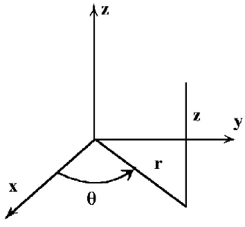
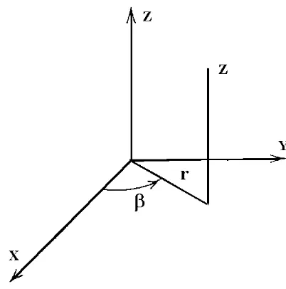
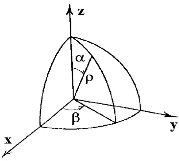
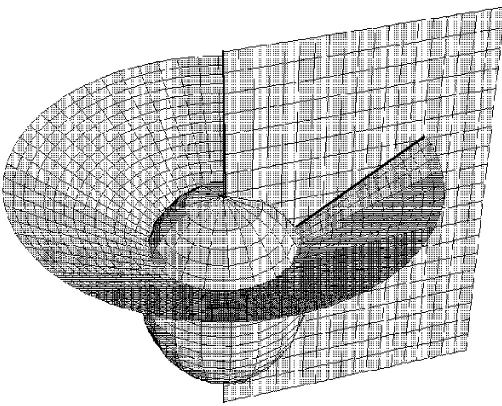
EXAMPLE 1.1-17. The following is an example of a set of transformation equations of the form defined by equations (1.1.7) and (1.1.8) in the case N = 3. Consider the transformation from cylindrical coordinates (r, α, z) to spherical coordinates (ρ, β, α).From the geometry of the figure 1.1-5 we can find the transformation equations
r=ρsinβ
α=α 0< α <2π z=ρcosβ 0< β < π
with inverse transformation
ρ=r2+z2
α=α β= arctan(r
z)
Now make the substitutions
Figure 1.1-5. Cylindrical and Spherical Coordinates The resulting transformations then have the forms of the equations (1.1.7) and (1.1.8).
Calculation of Derivatives
We now consider the chain rule applied to the differentiation of a function of the bar variables. We represent this differentiation in the indicial notation. Let Φ = Φ(x1, x2, . . . , xn) be a scalar function of the variablesxi, i= 1, . . . , N and let these variables be related to the set of variablesxi,withi= 1, . . . , N by
the transformation equations (1.1.7) and (1.1.8). The partial derivatives of Φ with respect to the variables
xi can be expressed in the indicial notation as
∂Φ
∂xi =
∂Φ
∂xj
∂xj ∂xi =
∂Φ
∂x1
∂x1 ∂xi +
∂Φ
∂x2
∂x2
∂xi +· · ·+
∂Φ
∂xN
∂xN
∂xi (1.1.9)
for any fixed value ofisatisfying 1≤i≤N.
The second partial derivatives of Φ can also be expressed in the index notation. Differentiation of equation (1.1.9) partially with respect toxmproduces
∂2Φ
∂xi∂xm =
∂Φ
∂xj
∂2xj
∂xi∂xm +
∂ ∂xm
∂Φ
∂xj
∂xj
∂xi. (1.1.10)
This result is nothing more than an application of the general rule for differentiating a product of two quantities. To evaluate the derivative of the bracketed term in equation (1.1.10) it must be remembered that the quantity inside the brackets is a function of the bar variables. Let
G= ∂Φ
∂xj =G(x
1, x2, . . . , xN)
to emphasize this dependence upon the bar variables, then the derivative ofGis
∂G ∂xm =
∂G ∂xk
∂xk ∂xm =
∂2Φ
∂xj∂xk
∂xk
∂xm. (1.1.11)
This is just an application of the basic rule from equation (1.1.9) with Φ replaced byG.Hence the derivative from equation (1.1.10) can be expressed
∂2Φ
∂xi∂xm =
∂Φ
∂xj ∂2xj
∂xi∂xm+
∂2Φ
∂xj∂xk
∂xj ∂xi
∂xk
∂xm (1.1.12)
EXAMPLE 1.1-18. Let Φ = Φ(r, θ) wherer, θare polar coordinates related to the Cartesian coordinates (x, y) by the transformation equationsx=rcosθ y=rsinθ.Find the partial derivatives∂Φ
∂x and ∂2Φ
∂x2 Solution: The partial derivative of Φ with respect toxis found from the relation (1.1.9) and can be written
∂Φ
The second partial derivative is obtained by differentiating the first partial derivative. From the product rule for differentiation we can write
∂2Φ
To further simplify (1.1.14) it must be remembered that the terms inside the brackets are to be treated as functions of the variablesrandθand that the derivative of these terms can be evaluated by reapplying the basic rule from equation (1.1.13) with Φ replaced by ∂Φ
∂r and then Φ replaced by ∂Φ
From the transformation equations we obtain the relationsr2=x2+y2 and tanθ= y
x and from
these relations we can calculate all the necessary derivatives needed for the simplification of the equations (1.1.13) and (1.1.15). These derivatives are:
2r∂r
Therefore, the derivatives from equations (1.1.13) and (1.1.15) can be expressed in the form
∂Φ
and (1.1.12) there is produced the same results as above.
Vector Identities in Cartesian Coordinates
Employing the substitutions x1 = x, x2 =y, x3 = z, where superscript variables are employed and
denoting the unit vectors in Cartesian coordinates by e1, e2, e3, we illustrated how various vector operations
Gradient. In Cartesian coordinates the gradient of a scalar field is
gradφ=∂φ
∂xe1+ ∂φ ∂ye2+
∂φ ∂ze3.
The index notation focuses attention only on the components of the gradient. In Cartesian coordinates these components are represented using a comma subscript to denote the derivative
ej·gradφ=φ,j=
∂φ
∂xj, j= 1,2,3.
The comma notation will be discussed in section 4. For now we use it to denote derivatives. For example
φ,j=
∂φ
∂xj, φ,jk=
∂2φ
∂xj∂xk, etc.
Divergence. In Cartesian coordinates the divergence of a vector field A is a scalar field and can be
represented
∇ ·A =div A= ∂A1
∂x + ∂A2
∂y + ∂A3
∂z .
Employing the summation convention and index notation, the divergence in Cartesian coordinates can be represented
∇ ·A =div A=Ai,i=
∂Ai
∂xi =
∂A1
∂x1 +
∂A2
∂x2 +
∂A3
∂x3
where iis the dummy summation index.
Curl. To represent the vector B = curlA = ∇ ×A in Cartesian coordinates, we note that the index
notation focuses attention only on the components of this vector. The componentsBi, i= 1,2,3 ofB can
be represented
Bi= ei·curlA=eijkAk,j, for i, j, k= 1,2,3
whereeijkis the permutation symbol introduced earlier andAk,j= ∂A∂xkj.To verify this representation of the
curlA we need only perform the summations indicated by the repeated indices. We have summing onjthat
Bi =ei1kAk,1+ei2kAk,2+ei3kAk,3.
Now summing each term on the repeated indexk gives us
Bi=ei12A2,1+ei13A3,1+ei21A1,2+ei23A3,2+ei31A1,3+ei32A2,3
Here iis a free index which can take on any of the values 1,2 or 3.Consequently, we have For i= 1, B1=A3,2−A2,3= ∂A3
∂x2 −
∂A2
∂x3
For i= 2, B2=A1,3−A3,1=
∂A1
∂x3 −
∂A3
∂x1
For i= 3, B3=A2,1−A1,2=
∂A2
∂x1 −
∂A1
∂x2
Other Operations. The following examples illustrate how the index notation can be used to represent
additional vector operators in Cartesian coordinates.
1. In index notation the components of the vector (B · ∇)A are
{(B · ∇)A} · ep=Ap,qBq p, q= 1,2,3
This can be verified by performing the indicated summations. We have by summing on the repeated index q
Ap,qBq=Ap,1B1+Ap,2B2+Ap,3B3.
The indexpis now a free index which can have any of the values 1,2 or 3.We have: for p= 1, A1,qBq =A1,1B1+A1,2B2+A1,3B3
=∂A1
∂x1B1+
∂A1
∂x2B2+
∂A1
∂x3B3
for p= 2, A2,qBq =A2,1B1+A2,2B2+A2,3B3
=∂A2
∂x1B1+
∂A2
∂x2B2+
∂A2
∂x3B3
for p= 3, A3,qBq =A3,1B1+A3,2B2+A3,3B3
=∂A3
∂x1B1+
∂A3
∂x2B2+
∂A3
∂x3B3
2. The scalar (B · ∇)φhas the following form when expressed in the index notation: (B · ∇)φ=Biφ,i=B1φ,1+B2φ,2+B3φ,3
=B1
∂φ ∂x1 +B2
∂φ ∂x2 +B3
∂φ ∂x3.
3. The components of the vector (B × ∇)φis expressed in the index notation by
ei·
(B × ∇)φ=eijkBjφ,k.
This can be verified by performing the indicated summations and is left as an exercise. 4. The scalar (B × ∇)·A may be expressed in the index notation. It has the form
(B × ∇)·A =eijkBjAi,k.
This can also be verified by performing the indicated summations and is left as an exercise. 5. The vector components of∇2A in the index notation are represented
ep· ∇2A =Ap,qq.
EXAMPLE 1.1-19. In Cartesian coordinates prove the vector identity curl (f A) =∇ ×(f A) = (∇f)×A+f(∇ ×A).
Solution: LetB = curl (f A) and write the components as
Bi=eijk(f Ak),j
=eijk[f Ak,j+f,jAk]
=f eijkAk,j+eijkf,jAk.
This index form can now be expressed in the vector form
B= curl (f A) =f(∇ ×A) + (∇f)×A
EXAMPLE 1.1-20. Prove the vector identity∇ ·(A+B) =∇ ·A+∇ ·B
Solution: Let A+B =C and write this vector equation in the index notation asAi+Bi =Ci. We then
have
∇ ·C =Ci,i= (Ai+Bi),i=Ai,i+Bi,i=∇ ·A+∇ ·B.
EXAMPLE 1.1-21. In Cartesian coordinates prove the vector identity (A· ∇)f =A· ∇f
Solution: In the index notation we write
(A· ∇)f =Aif,i=A1f,1+A2f,2+A3f,3
=A1
∂f ∂x1 +A2
∂f ∂x2 +A3
∂f
∂x3 =A· ∇f. EXAMPLE 1.1-22. In Cartesian coordinates prove the vector identity
∇ ×(A×B) =A(∇ ·B)−B(∇ ·A) + (B · ∇)A−(A· ∇)B
Solution: Thepthcomponent of the vector∇ ×(A×B) is
ep·[∇ ×(A×B)] =epqk[ekjiAjBi],q
=epqkekjiAjBi,q+epqkekjiAj,qBi
By applying the e−δidentity, the above expression simplifies to the desired result. That is,
ep·[∇ ×(A×B)] = (δpjδqi−δpiδqj)AjBi,q+ (δpjδqi−δpiδqj)Aj,qBi
=ApBi,i−AqBp,q+Ap,qBq−Aq,qBp
In vector form this is expressed
EXAMPLE 1.1-23. In Cartesian coordinates prove the vector identity∇ ×(∇ ×A) =∇(∇ ·A)− ∇2A
Solution: We have for theithcomponent of∇ ×A is given by ei·[∇ ×A] =eijkAk,j and consequently the
pthcomponent of∇ ×(∇ ×A) is
ep·[∇ ×(∇ ×A)] =epqr[erjkAk,j],q
=epqrerjkAk,jq.
Thee−δidentity produces
ep·[∇ ×(∇ ×A)] = (δpjδqk−δpkδqj)Ak,jq
=Ak,pk−Ap,qq.
Expressing this result in vector form we have∇ ×(∇ ×A) =∇(∇ ·A)− ∇2A. Indicial Form of Integral Theorems
The divergence theorem, in both vector and indicial notation, can be written
V
div·F dτ =
S
F·ndσ
V
Fi,idτ =
S
Finidσ i= 1,2,3 (1.1.16)
whereni are the direction cosines of the unit exterior normal to the surface,dτ is a volume element anddσ
is an element of surface area. Note that in using the indicial notation the volume and surface integrals are to be extended over the range specified by the indices. This suggests that the divergence theorem can be applied to vectors inn−dimensional spaces.
The vector form and indicial notation for the Stokes theorem are
S
(∇ ×F)·ndσ=
C
F·dr
S
eijkFk,jnidσ=
C
Fidxi i, j, k= 1,2,3 (1.1.17)
and the Green’s theorem in the plane, which is a special case of the Stoke’s theorem, can be expressed
∂F
2
∂x − ∂F1
∂y
dxdy=
C
F1dx+F2dy
S
e3jkFk,jdS=
C
Fidxi i, j, k= 1,2 (1.1.18)
Other forms of the above integral theorems are
V ∇
φ dτ=
S
φndσ
obtained from the divergence theorem by letting F =φ C whereC is a constant vector. By replacing F by
F×C in the divergence theorem one can derive
V
∇ ×Fdτ =−
S
F×n dσ.
In the divergence theorem make the substitutionF =φ∇ψto obtain
V
(φ∇2ψ+ (∇φ)·(∇ψ)dτ =
S
The Green’s identity
V
φ∇2ψ−ψ∇2φdτ =
S
(φ∇ψ−ψ∇φ)·ndσ
is obtained by first lettingF =φ∇ψin the divergence theorem and then lettingF =ψ∇φin the divergence theorem and then subtracting the results.
Determinants, Cofactors
ForA= (aij), i, j= 1, . . . , nann×nmatrix, the determinant ofA can be written as
detA=|A|=ei1i2i3...ina1i1a2i2a3i3. . . anin.
This gives a summation of then! permutations of products formed from the elements of the matrixA. The result is a single number called the determinant ofA.
EXAMPLE 1.1-24. In the casen= 2 we have
|A|=
aa1121 aa1222
=enma1na2m
=e1ma11a2m+e2ma12a2m
=e12a11a22+e21a12a21
=a11a22−a12a21
EXAMPLE 1.1-25. In the casen= 3 we can use either of the notations
A=
a11 a12 a13
a21 a22 a23
a31 a32 a33
or A=
a1
1 a12 a13
a2
1 a22 a23
a3
1 a32 a33
and represent the determinant ofAin any of the forms
detA=eijka1ia2ja3k
detA=eijkai1aj2ak3
detA=eijkai1aj2ak3
detA=eijka1ia2ja3k.
These represent row and column expansions of the determinant.
An important identity results if we examine the quantity Brst =eijkariajsakt. It is an easy exercise to
change the dummy summation indices and rearrange terms in this expression. For example,
Brst=eijkairajsakt =ekjiakrajsait=ekjiaitajsakr=−eijkaitajsakr =−Btsr,
and by considering other permutations of the indices, one can establish that Brst is completely
skew-symmetric. In the exercises it is shown that any third order completely skew-symmetric system satisfies
Brst=B123erst.ButB123= detAand so we arrive at the identity
Other forms of this identity are
eijkariasjatk=|A|erst and eijkairajsakt=|A|erst. (1.1.19)
Consider the representation of the determinant
|A|=
a1
1 a12 a13
a2
1 a22 a23
a3
1 a32 a33
by use of the indicial notation. By column expansions, this determinant can be represented
|A|=erstar1as2at3 (1.1.20)
and if one uses row expansions the determinant can be expressed as
|A|=eijka1ia2ja3k. (1.1.21)
DefineAi
mas the cofactor of the elementami in the determinant|A|.From the equation (1.1.20) the cofactor
ofar
1 is obtained by deleting this element and we find
A1r=erstas2at3. (1.1.22)
The result (1.1.20) can then be expressed in the form
|A|=ar1Ar1=a11A11+a21A12+a31A13. (1.1.23)
That is, the determinant|A|is obtained by multiplying each element in the first column by its corresponding cofactor and summing the result. Observe also that from the equation (1.1.20) we find the additional cofactors
A2
s=erstar1at3 and A3t =erstar1as2. (1.1.24)
Hence, the equation (1.1.20) can also be expressed in one of the forms
|A|=as2A2s=a12A21+a22A22+a32A23
|A|=at3A3t=a13A31+a23A32+a33A33
The results from equations (1.1.22) and (1.1.24) can be written in a slightly different form with the indicial notation. From the notation for a generalized Kronecker delta defined by
eijke
lmn=δlmnijk ,
the above cofactors can be written in the form
A1r=e123erstas2at3=
1 2!e
1jke
rstasjatk=
1 2!δ
1jk rstasjatk
A2r=e123esrtas1at3=
1 2!e
2jke
rstasjatk=
1 2!δ
2jk rstasjatk
A3r=e123etsrat1as2=
1 2!e
3jke
rstasjatk=
1 2!δ
These cofactors are then combined into the single equation
Air=
1 2!δ
ijk
rstasjatk (1.1.25)
which represents the cofactor of ar
i. When the elements from any row (or column) are multiplied by their
corresponding cofactors, and the results summed, we obtain the value of the determinant. Whenever the elements from any row (or column) are multiplied by the cofactor elements from a different row (or column), and the results summed, we get zero. This can be illustrated by considering the summation
amrAim=
1 2!δ
ijk
mstasjatkamr =
1 2!e
ijke
mstamrasjatk
= 1 2!e
ijke
rjk|A|=
1 2!δ
ijk
rjk|A|=δr|i A|
Here we have used the e−δidentity to obtain
δijkrjk=eijke
rjk=ejikejrk=δirδkk−δkiδkr = 3δir−δri = 2δri
which was used to simplify the above result.
As an exercise one can show that an alternate form of the above summation of elements by its cofactors is
armAmi =|A|δri.
EXAMPLE 1.1-26. In N-dimensions the quantityδj1j2...jN
k1k2...kN is called a generalized Kronecker delta. It
can be defined in terms of permutation symbols as
ej1j2...jNe
k1k2...kN =δ
j1j2...jN
k1k2...kN (1.1.26)
Observe that
δj1j2...jN
k1k2...kNe
k1k2...kN = (N!)ej1j2...jN
This follows becauseek1k2...kN is skew-symmetric in all pairs of its superscripts. The left-hand side denotes
a summation ofN! terms. The first term in the summation has superscriptsj1j2. . . jN and all other terms
have superscripts which are some permutation of this ordering with minus signs associated with those terms having an odd permutation. Because ej1j2...jN is completely skew-symmetric we find that all terms in the
EXERCISE 1.1
◮1. Simplify each of the following by employing the summation property of the Kronecker delta. Perform
sums on the summation indices only if your are unsure of the result. (a) eijkδkn
(b) eijkδisδjm
(c) eijkδisδjmδkn
(d) aijδin
(e) δijδjn
(f) δijδjnδni
◮2. Simplify and perform the indicated summations over the range 1,2,3
(a) δii
(b) δijδij
(c) eijkAiAjAk
(d) eijkeijk
(e) eijkδjk
(f) AiBjδji−BmAnδmn
◮3. Express each of the following in index notation. Be careful of the notation you use. Note thatA=Ai
is an incorrect notation because a vector can not equal a scalar. The notationA·ei=Aishould be used to
express theithcomponent of a vector. (a) A·(B ×C)
(b) A×(B ×C)
(c) B(A·C)
(d) B(A·C)−C(A·B)
◮4. Show theepermutation symbol satisfies: (a) eijk =ejki =ekij (b) eijk =−ejik=−eikj=−ekji ◮5. Use index notation to verify the vector identityA×(B ×C) =B(A·C)−C(A·B)
◮6. Letyi=aijxj andxm=aimzi where the range of the indices is 1,2
(a) Solve foryi in terms ofzi using the indicial notation and check your result
to be sure that no index repeats itself more than twice. (b) Perform the indicated summations and write out expressions
fory1, y2 in terms ofz1, z2
(c) Express the above equations in matrix form. Expand the matrix equations and check the solution obtained in part (b).
◮7. Use thee−δidentity to simplify (a) eijkejik (b) eijkejki ◮8. Prove the following vector identities:
(a) A·(B ×C) =B ·(C ×A) =C ·(A×B) triple scalar product (b) (A×B)×C =B(A·C)−A(B ·C)
◮9. Prove the following vector identities:
◮10. ForA = (1,−1,0) and B = (4,−3,2) find using the index notation,
(a) Ci=eijkAjBk, i= 1,2,3
(b) AiBi
(c) What do the results in (a) and (b) represent?
◮11. Represent the differential equations dy1
dt =a11y1+a12y2 and
dy2
dt =a21y1+a22y2
using the index notation.
◮12.
Let Φ = Φ(r, θ) wherer, θ are polar coordinates related to Cartesian coordinates (x, y) by the transfor-mation equations x=rcosθ and y=rsinθ.
(a) Find the partial derivatives ∂Φ
∂y, and
∂2Φ
∂y2
(b) Combine the result in part (a) with the result from EXAMPLE 1.1-18 to calculate the Laplacian
∇2Φ = ∂2Φ
∂x2 +
∂2Φ
∂y2
in polar coordinates.
◮13. (Index notation) Leta11= 3, a12= 4, a21= 5, a22= 6.
Calculate the quantityC=aijaij, i, j= 1,2.
◮14. Show the moments of inertiaIij defined by
I11=
R
(y2+z2)ρ(x, y, z)dτ I22=
R
(x2+z2)ρ(x, y, z)dτ I33=
R
(x2+y2)ρ(x, y, z)dτ
I23=I32=−
R
yzρ(x, y, z)dτ I12=I21=−
R
xyρ(x, y, z)dτ I13=I31=−
R
xzρ(x, y, z)dτ,
can be represented in the index notation as Iij = R
xmxmδ
ij−xixj
ρ dτ, where ρ is the density,
x1=x, x2=y, x3=z anddτ =dxdydzis an element of volume.
◮15. Determine if the following relation is true or false. Justify your answer.
ei·(ej×ek) = (ei×ej)· ek =eijk, i, j, k= 1,2,3.
Hint: Let em= (δ1m, δ2m, δ3m).
◮16. Without substituting values fori, l= 1,2,3 calculate all nine terms of the given quantities
(a) Bil= (δijAk+δkiAj)ejkl (b) Ail= (δmi Bk+δikBm)emlk
◮18.
Hint: Use the result from example 1.1-9.
◮20.
x) is the Jacobian determinant
of the transformation (1.1.7).
◮21. A third order systemaℓmnwithℓ, m, n= 1,2,3 is said to be symmetric in two of its subscripts if the
components are unaltered when these subscripts are interchanged. Whenaℓmnis completely symmetric then
aℓmn =amℓn =aℓnm =amnℓ =anmℓ =anℓm.Whenever this third order system is completely symmetric,
then: (i) How many components are there? (ii) How many of these components are distinct? Hint: Consider the three cases (i)ℓ=m=n (ii) ℓ=m=n (iii) ℓ=m=n.
◮22. A third order systembℓmn withℓ, m, n= 1,2,3 is said to be skew-symmetric in two of its subscripts
if the components change sign when the subscripts are interchanged. A completely skew-symmetric third order system satisfies bℓmn =−bmℓn = bmnℓ =−bnmℓ = bnℓm =−bℓnm. (i) How many components does
a completely skew-symmetric system have? (ii) How many of these components are zero? (iii) How many components can be different from zero? (iv) Show that there is one distinct component b123 and that
◮26. (Generalized Kronecker delta) Define the generalized Kronecker delta as then×ndeterminant
δij...kmn...p=
δi
m δni · · · δip
δj
m δnj · · · δjp
..
. ... . .. ...
δk
m δnk · · · δpk
whereδr
s is the Kronecker delta.
(a) Show eijk=δijk123
(b) Show eijk=δijk123
(c) Show δmnij =eijemn
(d) Define δrs
mn=δrspmnp (summation onp)
and show δmnrs =δmrδns−δrnδms
Note that by combining the above result with the result from part (c)
we obtain the two dimensional form of thee−δidentity ersemn=δmrδns−δnrδms.
(e) Defineδr m= 12δ
rn
mn (summation onn) and show δrstpst= 2δpr
(f) Show δrst rst = 3!
◮27. LetAirdenote the cofactor ofari in the determinant
a1
1 a12 a13
a2
1 a22 a23
a3
1 a32 a33
as given by equation (1.1.25).
(a) Show erstAir=eijkasjatk (b) Show erstAri =eijkajsakt
◮28. (a) Show that ifAijk =Ajik,i, j, k = 1,2,3 there is a total of 27 elements, but only 18 are distinct.
(b) Show that fori, j, k= 1,2, . . . , N there areN3 elements, but onlyN2(N+ 1)/2 are distinct.
◮29. Letaij =BiBj fori, j= 1,2,3 whereB1, B2, B3 are arbitrary constants. Calculate det(aij) =|A|. ◮30.
(a) For A= (aij), i, j= 1,2,3, show |A|=eijkai1aj2ak3.
(b) For A= (aij), i, j= 1,2,3, show |A|=eijkai1a
j
2ak3.
(c) For A= (aji), i, j= 1,2,3, show |A|=eijka1ia2ja3k.
(d) For I= (δi
j), i, j= 1,2,3, show |I|= 1.
◮31. Let |A| = eijkai1aj2ak3 and define Aim as the cofactor of aim. Show the determinant can be
expressed in any of the forms:
(a) |A|=Ai1ai1 where Ai1=eijkaj2ak3
(b) |A|=Aj2aj2 where Ai2=ejikaj1ak3
◮32. Show the results in problem 31 can be written in the forms:
◮37. Simplify the expressions:
(a) (Aijkl+Ajkli+Aklij +Alijk)xixjxkxl
Hint: Use the results from problem 39.
◮42. Determine if the following statement is true or false. Justify your answer. eijkAiBjCk=eijkAjBkCi. ◮43. Letaij, i, j= 1,2 denote the components of a 2×2 matrixA,which are functions of timet.
(a) Expand both|A|=eijai1aj2 and|A|=
a11 a12
a21 a22
to verify that these representations are the same.
(b) Verify the equivalence of the derivative relations
d|A|
dt =eij dai1
dt aj2+eijai1 daj2
dt and d|A|
dt =
da11
dt da12
dt
a21 a22 +
daa1121 a12
dt da22
dt
(c) Letaij, i, j= 1,2,3 denote the components of a 3×3 matrixA,which are functions of timet.Develop
appropriate relations, expand them and verify, similar to parts (a) and (b) above, the representation of a determinant and its derivative.
◮44. Forf =f(x1, x2, x3) andφ=φ(f) differentiable scalar functions, use the indicial notation to find a
formula to calculate gradφ .
◮45. Use the indicial notation to prove (a) ∇ × ∇φ=0 (b) ∇ · ∇ ×A = 0 ◮46. IfAij is symmetric andBij is skew-symmetric,i, j= 1,2,3, then calculateC=AijBij.
◮47. AssumeAij =Aij(x1, x2, x3) andAij =Aij(x1, x2, x3) fori, j = 1,2,3 are related by the expression
Amn=Aij
∂xi
∂xm
∂xj
∂xn.Calculate the derivative
∂Amn
∂xk .
◮48. Prove that if any two rows (or two columns) of a matrix are interchanged, then the value of the
determinant of the matrix is multiplied by minus one. Construct your proof using 3×3 matrices.
◮49. Prove that if two rows (or columns) of a matrix are proportional, then the value of the determinant
of the matrix is zero. Construct your proof using 3×3 matrices.
◮50. Prove that if a row (or column) of a matrix is altered by adding some constant multiple of some other
row (or column), then the value of the determinant of the matrix remains unchanged. Construct your proof using 3×3 matrices.
◮51. Simplify the expressionφ=eijkeℓmnAiℓAjmAkn.
◮52. LetAijk denote a third order system wherei, j, k= 1,2.(a) How many components does this system
have? (b) Let Aijk be skew-symmetric in the last pair of indices, how many independent components does
the system have?
◮53. Let Aijk denote a third order system where i, j, k = 1,2,3. (a) How many components does this
system have? (b) In addition let Aijk = Ajik and Aikj = −Aijk and determine the number of distinct
◮54. Show that every second order systemTijcan be expressed as the sum of a symmetric systemAij and
skew-symmetric systemBij. FindAij andBij in terms of the components ofTij.
◮55. Consider the systemAijk, i, j, k= 1,2,3,4.
(a) How many components does this system have?
(b) AssumeAijk is skew-symmetric in the last pair of indices, how many independent components does this
system have?
(c) Assume that in addition to being skew-symmetric in the last pair of indices,Aijk+Ajki+Akij= 0 is
satisfied for all values ofi, j,andk,then how many independent components does the system have?
◮56. (a) Write the equation of a line r =r0+t Ain indicial form. (b) Write the equation of the plane
n·(r−r0) = 0 in indicial form. (c) Write the equation of a general line in scalar form. (d) Write the
equation of a plane in scalar form. (e) Find the equation of the line defined by the intersection of the planes 2x+ 3y+ 6z = 12 and 6x+ 3y+z = 6. (f) Find the equation of the plane through the points (5,3,2), (3,1,5), (1,3,3).Find also the normal to this plane.
◮57. The angle 0≤θ≤π between two skew lines in space is defined as the angle between their direction
vectors when these vectors are placed at the origin. Show that for two lines with direction numbersai and
bi i= 1,2,3, the cosine of the angle between these lines satisfies
cosθ= √ aibi
aiai√bibi
◮58. Letaij =−aji fori, j= 1,2, . . . , N and prove that forN odddet(aij) = 0. ◮59. Letλ=Aijxixj whereAij =Aji and calculate (a) ∂λ
∂xm
(b) ∂
2λ
∂xm∂xk
◮60. Given an arbitrary nonzero vectorUk,k= 1,2,3, define the matrix elementsaij=eijkUk, whereeijk
is the e-permutation symbol. Determine if aij is symmetric or skew-symmetric. SupposeUk is defined by
the above equation for arbitrary nonzeroaij, then solve forUk in terms of theaij.
◮61. If Aij = AiBj = 0 for all i, j values andAij =Aji fori, j = 1,2, . . . , N, show thatAij = λBiBj
where λis a constant. State whatλis.
◮62. Assume thatAijkm, withi, j, k, m= 1,2,3,is completely skew-symmetric. How many independent
components does this quantity have?
◮63. Consider Rijkm,i, j, k, m = 1,2,3,4. (a) How many components does this quantity have? (b) If
Rijkm =−Rijmk=−Rjikm then how many independent components doesRijkm have? (c) If in addition
Rijkm=Rkmij determine the number of independent components.
◮64. Letxi=aijx¯j, i, j= 1,2,3 denote a change of variables from a barred system of coordinates to an
unbarred system of coordinates and assume that ¯Ai=aijAj whereaij are constants, ¯Ai is a function of the
¯
xj variables andAj is a function of thexj variables. Calculate ∂
¯
Ai
∂x¯m