Optimasi Hidrolisis Selulosa dari Tandan Kosong Kelapa Sawit menjadi Selulosa Mikrokristal dan Aplikasi sebagai Pengisi pada Komposit Polimer Termoplastik Pati Singkong

(1)

LAMPIRAN A

RANCANGAN DAN ANALISIS PERCOBAAN DENGAN

METODE RESPONSE SURFACE MENGGUNAKAN

MINITAB 16 SOFTWARE

LA-1 Rancangan Percobaan Optimasi Hidrolisis Selulosa dari Tandan Kosong

Kelapa Sawit

Rancangan percobaan menggunakan metode

Response Surface Methode

(RSM) dengan 3 variabel bebas (Ferreira, et.al, 2007), dimana variabel bebas, k = 3,

maka

Central Composite Design

dengan 3 faktor (variabel):

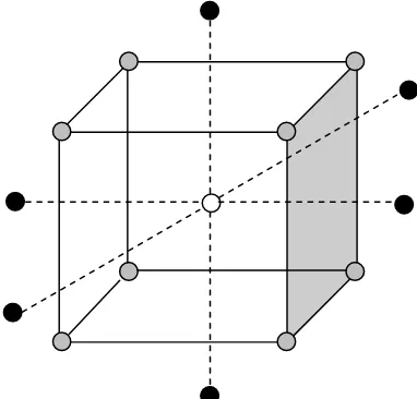
Gambar LA-1

Central Composite Design

untuk 3 Faktor

(Ferreira, et.al, 2007)

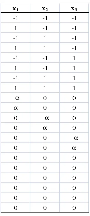
Dengan perulangan 6 kali pada titik tengah, maka matriks

Central Composite

Design

terlihat pada Tabel LA-1, dimana :

682 ,

1

2

4 3 4 k

=

(2)

Tabel LA-1 Matriks

Central Composite Design

x

₁

x

₂

x

₃

-1

1 -1

-1

1 -1

1

1 -1

-1

1

1 -1

1

1 −α

0

0 α

₀

0 −α

0

0 α

₀

0

0 −α

0

0 α

0

0 LA-2 Rancangan Percobaan Optimasi dalam

Minitab 16 Statistical Software

(3)

1. Memilih Stat

→

DOE

→

Response Surface

→

Create Response Surface Design

Layar monitor memperlihatkan kotak dialog

Create Response Surface Design

(Gambar LA-2).

Gambar LA-2 Kotak Dialog

Create Response Surface

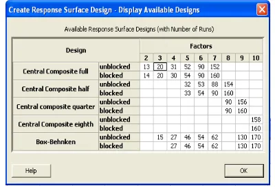
2. Memilih tipe desain

Central Composite

dengan jumlah faktor sebanyak 3 faktor,

kemudian memilih

Display Available Designs

sehingga layar monitor

memperlihatkan kotak dialog

Response Surface Design-Display Available

Designs

(Gambar LA-3).

(4)

3. Memilih

Central Composite Full Unblocked

untuk 3 faktor, diperoleh 20

pengamatan kemudian memilih OK, untuk kembali ke menu sebelumnya dan

memillih

Design

sehingga layar monitor memperlihatkan kotak dialog

Create

Response Surface Design-Designs

(Gambar LA-4).

Gambar LA-4 Kotak Dialog

Create Response Surface Design-Designs

(5)

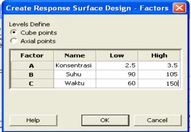
5. Memilih

cube points

untuk

levels define

, kemudian mengisi nama faktor serta

level minimum dan maksimum masing-masing faktor. Selanjutnya, kembali ke

menu sebelumnya dan memilih

options

sehingga layar monitor memperlihatkan

kotak dialog

Create Response Surface Design-Factors

(Gambar LA-6).

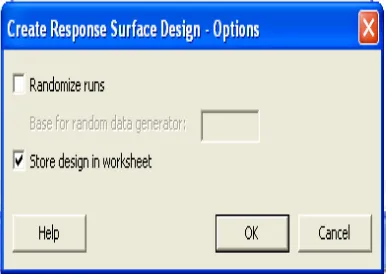
Gambar LA-6 Kotak Dialog

Create Response Surface Design-Options

6. Menghilangkan tanda cek pada

randomize runs

dan kembali ke menu

sebelumnya dan memilih OK, sehingga

output

muncul dalam 2

window

, yaitu

(6)

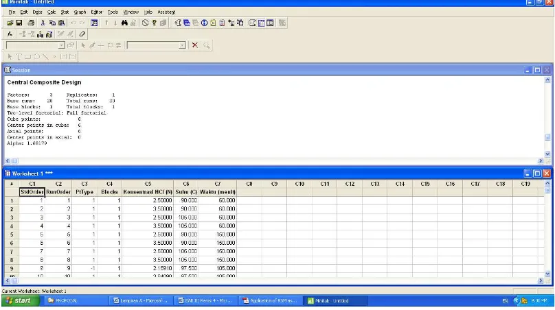
Gambar LA-7 Hasil Desain

Response Surface

7. Nama dan data variabel respon (derajat kristalinitas) selanjutnya diisikan pada

kolom C8

worksheet

, kemudian

worksheet

disimpan dengan nama file tertentu.

LA-3 Analisis Percobaan Optimasi dalam

Minitab 16 Statistical Software

Berdasarkan data response yang telah diinput pada kolom C8

worksheet

dilakukan analisis data

response surface

dengan langkah-langkah sebagai berikut:

1. Memilih Stat

→

DOE

→

Response Surface

→

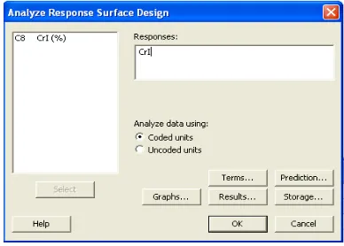
Analyze Response Surface

Layar monitor memperlihatkan kotak dialog

Analyze Response Surface Design

(7)

Gambar LA-8 Kotak Dialog

Analyze Response Surface

2. Memilih

graphs

, sehingga layar monitor memperlihatkan kotak dialog

Analyze

Response Surface Design-Graphs

(Gambar LA-9). Selanjutnya, memilih

regular

untuk

residual for plots

serta memberi tanda cek pada

residuals for fits

dan

residals versus ordered

. Perintah ini berfungsi membuat plot residual dengan

taksiran model dam plot residual dengan data yang bermanfaat untuk memeriksa

kecukupan model.

Gambar LA-9 Kotak Dialog

Analyze Response Surface

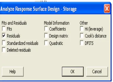
3. Memilih

Storage

sehingga layar monitor akan memperlihatkan kotak dialog

(8)

cek pada

residuals

dan memilih OK. Layar monitor akan kembali ke menu

sebelumnya, kemudian memilih OK.

Gambar LA-10 Kotak Dialog

Analyze Response Surface-Storage

(9)

(10)

Konsentrasi HCl (N) 12,78 0,005 Suhu (C) 12,83 0,005 Waktu (menit) 29,47 0,000 Square 1,89 0,195 Konsentrasi HCl (N)*Konsentrasi HCl (N) 1,22 0,296 Suhu (C)*Suhu (C) 0,04 0,847 Waktu (menit)*Waktu (menit) 4,88 0,052 Interaction 3,15 0,073 Konsentrasi HCl (N)*Suhu (C) 2,12 0,176 Konsentrasi HCl (N)*Waktu (menit) 6,55 0,028 Suhu (C)*Waktu (menit) 0,78 0,398 Residual Error

Lack-of-Fit 28,68 0,001 Pure Error

Total

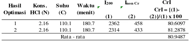
Unusual Observations for CrI

Obs StdOrder CrI Fit SE Fit Residual St Resid 1 1 75,192 75,881 0,446 -0,689 -2,20 R 5 5 78,180 78,808 0,446 -0,628 -2,00 R 9 9 78,704 77,850 0,425 0,854 2,50 R 11 11 79,039 78,216 0,425 0,823 2,41 R

R denotes an observation with a large standardized residual.

Estimated Regression Coefficients for CrI using data in uncoded units

Term Coef Constant 21,1004 Konsentrasi HCl (N) 14,4551 Suhu (C) 0,446454 Waktu (menit) 0,165496 Konsentrasi HCl (N)* -0,633377 Konsentrasi HCl (N)

Suhu (C)*Suhu (C) -5,05223E-04 Waktu (menit)*Waktu (menit) -1,56522E-04 Konsentrasi HCl (N)*Suhu (C) -0,0748745 Konsentrasi HCl (N)*Waktu (menit) -0,0219089 Suhu (C)*Waktu (menit) -5,03718E-04

(11)