HYPOTHESIS TESTING ON ENVIRONMENTAL KUZNETS CURVE OF
AGRICULTURAL SECTOR IN JAVA ISLAND: PANEL DATA ANALYSIS
Pengujian Hipotesis Kurva Lingkungan Kuznets (Environmental Kuznets
Curve) Sektor Pertanian di Pulau Jawa : Analisis Data Panel
Ali Hasyim Al Rosyid1, Irham1,2, Jangkung Handoyo Mulyo1,3
1Student of Postgraduate Program of Faculty of Agriculture, Universitas Gadjah Mada Jl. Flora, Bulaksumur, Kec.Depok, Kabupaten Sleman,
Daerah Istimewa Yogyakarta 55281
2Asia-Pacifi c Study Centre (PSAP), Universitas Gadjah Mada Jl. Tevesia, Bulaksumur B-13, Yogyakarta 55281, Indonesia 3Population and Policy Studies Center (PSKK), UniversitasGadjahMada
Jl. Tevesia, Bulaksumur, Kec.Depok, Kabupaten Sleman, Daerah Istimewa Yogyakarta 55281
[email protected]; [email protected]; Diterima tanggal 6 Juni 2017 ; Disetujui tanggal 15 Juni 2017
ABSTRACT
One obstacle in the improvement of community welfare in the agricultural sector, especially in Java, is the environmental externality which constantly exists in every economic activity. The objective of this research was to estimate greenhouse gas emission coming from agricultural sector in Java and identify whether farmers in Java had allocated environmental conservation costs as the impact of greenhouse gas emission from agricultural activities in Java. The inventory method of greenhouse gas emission from agricultural sector is based on inventory guidelines published by IPCC (Intergovernmental Panel on Climate Change) in 2006. As for the analysis to determine the relationship between greenhouse gas emission and GRDP of agricultural subsector per agricultural labor, The Environmental Kuznets Curve (EKC) was employed, alongside greenhouse gas emission indicators representing environmental degradation and GRDP of agricultural subsector per agricultural worker representing of per capita income of agricultural. Overall, greenhouse gas emissions, both CH4 methane emissions and carbon dioxide emission (CO2) - produced from rice cultivation, fertilizer application, livestock enteric fermentation and poultry manure - are gradually increasing. And the relationship between greenhouse gas emission and GRDP per worker has inverted-U shape; and it is in line with EKC hypothesis. Thereby, the role of the entire community elements and government support in implementing mitigation technology and agricultural adaptation is needed to cope with impacts of greenhouse gas emission, such as climate change.
Keywords: Agricultural Sector, EKC (Environmental Kuznets Curve), GHG Emission (Greenhouse Gas)
INTISARI
konservasi lingkungan sebagai dampak emisi gas rumah kaca dari kegiatan pertanian di Jawa. Metode inventarisasi emisi gas rumah kaca dari sektor pertanian didasarkan pada pedoman inventarisasi yang diterbitkan oleh IPCC (Intergovernmental Panel on Climate Change) pada tahun 2006. Sedangkan untuk analisis untuk mengetahui hubungan antara emisi gas rumah kaca dan PDRB sektor pertanian per tenaga kerja pertanian, menggunakan Environmental Kuznets Curve (EKC) di samping itu digunakan indikator emisi gas rumah kaca yang mewakili degradasi lingkungan dan PDRB subsektor pertanian per pekerja pertanian yang merupakan pendekatan pendapatan per kapita pertanian. Secara keseluruhan, emisi gas rumah kaca, baik emisi metana CH4 dan emisi karbon dioksida (CO2) yang dihasilkan dari budidaya padi, aplikasi pupuk, fermentasi enterik ternak dan pupuk unggas meningkat secara bertahap. Hubungan antara emisi gas rumah kaca dan PDRB sektor pertanian per tenaga kerja pertanian seperti U-terbalik. sehingga sejalan dengan hipotesis EKC. Dengan demikian, peran seluruh elemen masyarakat dan dukungan pemerintah dalam menerapkan teknologi mitigasi dan adaptasi pertanian diperlukan untuk mengatasi dampak emisi gas rumah kaca, seperti perubahan iklim.
Kata Kunci: Emisi GRK (Gas Rumah Kaca), EKC (Environmental Kuznets Curve), Sektor Pertanian
environmental damage resulted from the production process of goods and services have never been considered. As a result, the price used in the market is way too low in comparison with the applied price – as the price does not include ‘environmental costs’.
As a key sector in the fulfi llment of food needs, emissions generated from the agricultural sector are expected to continue to keep rising until 2030, alongside increasing food demand. In order to handle this Indonesian Government has committed to reduce GHG emission by 26% by 2020. (Ariani et.al., 2016).
Dasgupta et.al. (2002) proposes the hypothesis used in this EKC: at the early stage of the industrialization process, pollution grows real swiftly because the main priority is to increase output, and the community tends to be more interested in getting jobs and having higher income, INTRODUCTION
A g r i c u l t u r e i n J a v a r e m a i n s as the dominant sector, viewed from its contributions to total GDP and the employment in this sector. If we view the agricultural sector’s GDP contribution in Indonesia, the agricultural sector contributes to Rp.441.601.433,4 (Billion) or equal to 36.50% out of total GDP of Indonesian agriculture sector.
rather than getting good environmental quality. According to Everett et al. (2010) the reversed-U curve illustrates the degree of environmental degradation will go together with increasing per capita national income. De Brunye, et al., (1998) believes that EKC does not happen in the long run. It is, therefore, the U-Shape will only happen at the early stage of the relationship between environmental damage level and per-capita income. In the condition above, a certain level of income will have a new turning point. Dinda (2004) and Song, et.al. (2008) develop EKC relationship in the form of cubic polynomials, where such model can be used to examine several relationship forms between environmental indicators and economic growth.
Environmental degradation becomes a hotly debated issue between economic experts and environmental experts. Lau et al. (2014) empirically tested the hypothesis of the Kuznets Environment Curve in Malaysia by looking at the relationship between Foreign Direct Investment and free trade system with CO2 emissions, viewed for its short and long term. Farhani et al., (2014) carried out a research to examine the hypothesis of Kuznets environmental curve in Middle East and North Africa countries using panel data from 1990-2010. The results demonstrate that the EKC model obtains inverted-U between environmental degradation and income per capita. Azam and Khan (2016)
undertook a research to estimate the Kuznets Environment Curve hypothesis for 4 countries. The use of OLS in this research is capable of proving the EKC hypotheses in countries with low income and rather low income. Wang et.al., (2016) performed a research to investigate impacts of economic growth and urbanization on level of sulfur dioxide in the air of China. The research results suggest the evidence of inverted-U relationship between economic growth and sulfur dioxide emissions. However, the relationship between urbanization and sulfur dioxide emission does not show relationship similar to inverted-U.
Apergis and Ozturk (2015) tested the hypothesis (Environmental Kuznets Curve) in 14 countries in Asia in 1990-2011. The results of the analysis show that per capita income has a significant and positive infl uence on CO2 emissions in 14 Asian countries studied, as well as population density also have an effect on emissions increase. In addition, the average economic growth in 14 countries in Asia is still in the early stages so that the increase in income per capita still has an impact on the increase of environmental pollution.
METHODS
The selection of research site was conducted purposively, taking location-specifi c condition into consideration. The reason for selecting Java for this research was based on the roles of agricultural sector, employment rate and its contribution to the national GDP. The provinces in Java have large percentage.
T h e d a t a w a s c o l l e c t e d b y documentation: the data used was recorded from the data sources or existing documents from 2001-2015 in fi ve province of Java Island. The documents were people’s notes or works on events in the past. The data employed in this research were those resulted from recordings in government agencies, such as East Java Provincial Government, Central Java Provincial Government, Yogyakarta Provincial Government, West Java Provincial Government and Banten Provincial Government; Central Statistics Agencies of East Java Province, Central Java Province, Yogyakarta Province, West Java Province, and Banten Province. In addition, other supporting data were also obtained from other institutions.
The Measurement of Greenhouse Gas
Emission (GRK) from Agricultural
Sector in Java
The inventory method of greenhouse gas emissions from the agricultural sector is based on the inventory guidelines published by IPCC (Intergovernmental
Panel on Climate Change) in 2006. The measurement methods are as follows:
a. Agriculture (Food Crops, Horticultures, and Plantations)
Emissions from agricultural sector especially food crops, horticultures and plantations can be approximated from CH4 emission from rice paddy cultivation and carbon dioxide resulted from urea fertilizers application. CH4 emissions are calculated by multiplying the daily emission factor by the length of rice cultivation and harvest area using the following equation (IPPC, 2006):
ECH4=LT x HT x EFfl ooded land x 10-3 Where:
E CH4 = CH4 emission of rice paddy (ton/ year)
RPA = Rice paddy planting area HT = In average total day, planting rice
paddy within a year (rice paddy harvest index in average is 220) EFfi eld = Emission factor of rice paddy
CH4 (1.3 kg CH4/ha/day) CO2 Emission of urea fertilizer can be calculated using equation below (IPPC, 2006):
CO2Emission = (MUreaxEFUrea) Where:
CO2-Emission = annual CO2 emission from Urea application (ton/year) MUrea = total urea fertilizer being applied
(ton/year)
Based on IPCC (Tier 1) for the urea emission factor is 0.20 or equivalent to C content of urea fertilizer based on atomic weight (20% of CO (NH2)2).
b. Livestock
G r e e n h o u s e g a s e m i s s i o n s i n livestock are calculated from methane emissions (CH4) generated from livestock enteric fermentation and methane emissions from livestock manure management. The estimation of CH4 emission level from livestock enteric fermentation uses the equation below (IPPC, 2006):
Emissions=EFTx NTx10-3 Where
Emissions = CH4 Emission from enteric fermentation (ton/year) EFT = CH4 Emission factor from
certain types of livestock (kg CH4/animal/year)
NT = total certain types/ categories of livestock slaughtered individually
Livestock manure does not only p r o d u c e f e c e s a n d u r i n e , b u t a l s o considerably high methane (CH4). The livestock manure potential to emit methane may occur during storage and even processing. This methane production process can occur and will increase if the environment is in anaerobic condition. The methane emission is strongly affected by types of feed, the quality of poultry feed
and livestock manure management. In the present research, methane emissions from livestock management used the formula from IPPC (2006) below (IPPC, 2006):
Where:
CH4 manure = CH4 Emission from livestock manure management (ton/ year)
EF(T) = CH4 Emission factor from certain types of livestock manure (kg CH4/animal/year) N(T) = Total certain category of
livestock being slaughtered (per animal)
T = Types or categories of livestock
The Analysis of Relationship between
E n v i ro n m e n t a l D e g r a d a t i o n a n d
Agricultural Sector GRDP per Worker
EKC shows that environmental degradation (greenhouse emissions) will increase in line with increasing per capita income, but if it has reached a certain point called turning-point, there will be decline in environmental degradation despite rising per capita income. Based on the above, the estimation that can be used to view the relationship between environmental degradation and per-capita income is: The Environmental Kuznets Curve (EKC) model with greenhouse gas emission indicators:
GHG = C + 1 GRDP ALit + 2 GRDP ALit2 +
Description:
GHGt = Total Green House Gas Emissions (CO2 and CH4 converted to CO2) from Agricultural Sector Activity (ton / year)
GRDP AL = Regional Domestic Income Bruto Per Agricultural Workers (rupiah)
C = Constant
E = Stochastic Disruption
B = Coeffi cient of independent variable
t = Year t
The research will be conducted using testing with three possible models in panel data analysis, namely OLS, fi xed effect, and random effect to get description on the difference of these three results. Further
best model selection was done through Chow Test, Breusch-Pagan, and Hausman.
Chow Test
The testing mechanism using Chow Test is described as follows (Gujarati, 2006);
Hypothesis:
H0 : α_1 = α_2 = … = α_i (similar intercept, no significant effects from cross section unit)
H1 : α_i ≠ 0; i = 1,2,…,n (at least there is one different intercept, a signifi cant effect is found in the cross section unit). If F_count > F_(α;[db]_1;[db]_2) or Probability value<α then H0 is rejected. That is, Fixed Effect Model is better than Common Effect Model.
Breusch-Pagan Test
Hausman Test
The testing mechanism takes after Wald’s criteria using statistical values that will follow the chi-square distribution below (Gujarati, 2006):
Hypothesis:
H0 : Correlation (X_(it,) _it ) = 0 (cross sectional effect is not related to other independent variables, REM is better than FEM)
H1 : Correlation (X_(it,) _it ) ≠ 0 (cross sectional effect is related to other independent variables, FEM is better than REM)
The decision over Hausman test is based on comparisons using the chi-square test. If the value of χ_obs2 > χ_tab2 or p-value is smaller than the signifi cance level specifi ed, H0 is rejected. That is, Fixed Effect Model is better than Random Effect Model.
RESULTS AND DISCUSSION
The Measurement of Greenhouse Gas
Emission (GRK) from Agricultural
Sector in Java
Global warming is the process of increasing the average temperature of the atmosphere, the ocean, and the Earth’s land caused by increasing concentrations of greenhouse gases due to human activities (Suarsana and Wahyuni, 2011). The Intergovernmental Panel on Climate Change (IPCC) has provided guidance to estimate Greenhouse Gas Emission
(GHG). The calculation method followed in IPCC guidelines for calculating GHG emissions or uptake is multiplication of human activity information within a certain period of time (activity data) and emissions or uptake per unit of activity (emission or uptake factors, FE).
Rice fields are ideal soils for cultivation for rice crops, either once a year or even throughout the year. Inundated soil is an ideal condition for producing methane (Sass and Cicerone, 1999). The practice of rice cultivation in rice fi elds also determines the level of methane produced and released into the atmosphere (Schutz et al., 1990). The fi gure below shows the development of methane emissions resulted from rice cultivation activities in Java in the period of 2001-2015.
The figure provides information related to CH4 methane emission from rice cultivation in Java. In the period 2001-2015, the emissions generated from the rice cultivation activities in Java have increased. The growth rate of methane emissions from rice paddy is 1.10% per year. This condition shows that the level of methane emission in 2015 is greater than the methane emission in 2001. The value of methane emissions (CH4) generated from rice cultivation in 2001 is 1,158,627 tons, whilst in 2013, it increases into 1,771,437 tons.
Java is determined by the area of rice cultivation (this research uses the harvested area approach). A number of mitigation technologies in the effort of reducing the level of methane emissions in rice paddy can be done by applying the system without tillage, replacing powdered urea fertilizer
with ammonium sulphate or tablet urea fertilizer, applying direct seeding plant (Wihadjaka, 2015), applying intermittent irrigation, and replacing rice varieties with superior rice variety and low emission (Kartikawati et.al., 2011).
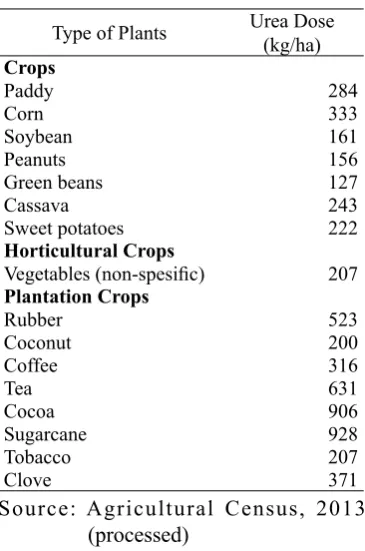
In addition to rice cultivation activities in the fi elds, urea fertilization application onto agricultural land may also lead to greenhouse gas emission, i.e. carbon dioxide gas (CO2). The urea fertilizer application on agricultural land has caused the release of CO2 trapped during the fertilizer production.
Based on the table 1 can be seen that in general the use of urea fertilizer by farmers exceeds the dose recommended by the ministry of agriculture. As a result a lot of actual fertilizer wasted because it is no longer needed by the plant. In addition, the excess N on the ground will also lead to increased production of methane on the ground. The use of inorganic fertilizers to be more effi cient should be based on the Figure 1. The development of the estimated value of methane emissions (CH4) from rice
fi eld cultivation activity in Java Island in 2001-2015.
Table 1. Urea Fertilizer Application in Each Type of Plants
Type of Plants Urea Dose (kg/ha)
Crops
Paddy 284
Corn 333
Soybean 161
Peanuts 156
Green beans 127
Cassava 243
Sweet potatoes 222
Horticultural Crops
Vegetables (non-spesifi c) 207
Plantation Crops
Rubber 523
Coconut 200
Coffee 316
Tea 631
Cocoa 906
Sugarcane 928
Tobacco 207
Clove 371
needs of the plant. This can be seen from leaf color i by using leaf color chart.
The figure displays information related to estimation of carbon dioxide (CO2) emissions resulted from urea fertilizer application in Java. In the period 2001-2015, carbon dioxide (CO2) emission from urea fertilizer application in Java Island has increased. The growth of carbon dioxide emission from urea fertilizer application is 0.48% per year. Based on this, it can be seen that value of carbon dioxide (CO2) emission resulted from fertilizer application in 2015 is higher (678,940 tons) in comparison with carbon dioxide emission at the same source in 2001 (726,301 tons).
The value of carbon dioxide emission (CO2) is determined by several components, including cultivation area (this research used the harvested area approach) for each crop. Besides, other components determining the level of carbon dioxide emission is the application dose of urea fertilization onto crops. Average farmers
apply fertilization dose, especially urea, which exceeds the dose recommended by the government. One of consequences is the greater emission of carbon dioxide yielded from urea fertilization activity.
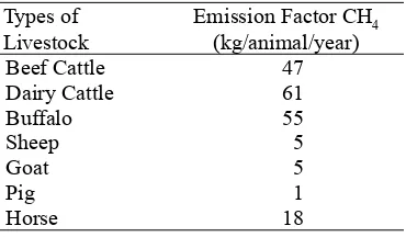
Based on the table 2, it is known that the CH4 emission factor value derived from the fermentation of the enteric of livestock is the most produced by the dairy cows at 61 kg /animal/ year. While the cattle that produce CH4 least seen from the emission factor of pigs with emission factor value of 1 kg / animal / year. This emission factor
Table 2. Value of CH4Emission Factor from Enteric Fermentation according to Livestock Types (EFT)
Types of Livestock
Emission Factor CH4 (kg/animal/year)
Beef Cattle 47
Dairy Cattle 61
Buffalo 55
Sheep 5
Goat 5
Pig 1
Horse 18
Source: IPCC, 2006
value is then multiplied by the existing livestock population in Java Island, so that will be obtained CH4 emission value from the fermentation of enteric cattle in each livestock each year.
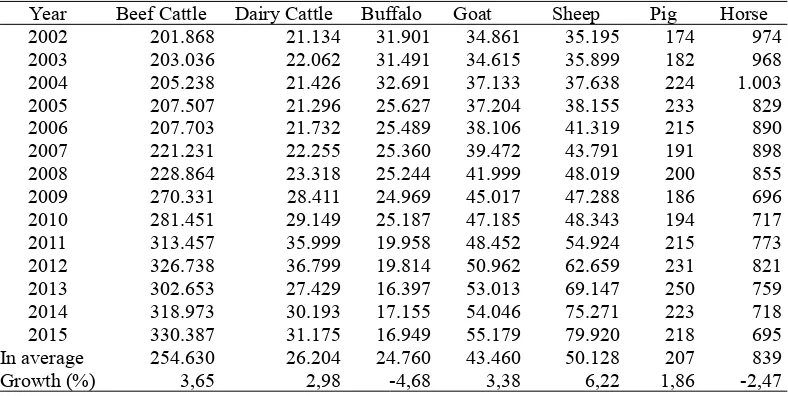
Based on the table 3, it can be seen that methane (CH4) in 2002 is mostly produced by enteric fermentation of beef cattle, i.e. 201,868 tons, whilst the livestock producing the least amount of methane (CH4) from enteric fermentation is 174 tons. Such condition remains unchanged by 2015. That is, methane emission from enteric fermentation of beef cattle still dominates the livestock methane emission contribution in terms of enteric fermentation in Java, whereas pigs contributes to smallest methane emission in Java in terms of livestock’s enteric fermentation. If viewed from the average number per year for each livestock, the
largest one is methane emissions (CH4) from beef cattle is 254,630 tons per year; while the smallest emission comes from pigs, by 207 tons per year .
Overall, the level of methane (CH4) emission from enteric fermentation of beef cattle in Java has increased by 3.65% per year. This value is in line with the increasing beef cattle population from 2002 to 2015. As for pigs, the positive growth happening is 1.86% per year. Buffalo and horse in Java experience the growth of negative methane (CH4) emission per year. It is parallel with the declining buffalo and horse population in Java. It happens because of the difficulties in providing suitable land for buffaloes and horses in Java, in addition to their more complicated raising methods - in comparison with beef cattle or sheep’s, making the breeders have less interest in raising buffalos and horses. Table 3. Estimates of Methane Emissions (CH4) from Livestock Enteric Fermentation (ton)
Year Beef Cattle Dairy Cattle Buffalo Goat Sheep Pig Horse 2002 201.868 21.134 31.901 34.861 35.195 174 974 2003 203.036 22.062 31.491 34.615 35.899 182 968 2004 205.238 21.426 32.691 37.133 37.638 224 1.003 2005 207.507 21.296 25.627 37.204 38.155 233 829 2006 207.703 21.732 25.489 38.106 41.319 215 890 2007 221.231 22.255 25.360 39.472 43.791 191 898 2008 228.864 23.318 25.244 41.999 48.019 200 855 2009 270.331 28.411 24.969 45.017 47.288 186 696 2010 281.451 29.149 25.187 47.185 48.343 194 717 2011 313.457 35.999 19.958 48.452 54.924 215 773 2012 326.738 36.799 19.814 50.962 62.659 231 821 2013 302.653 27.429 16.397 53.013 69.147 250 759 2014 318.973 30.193 17.155 54.046 75.271 223 718 2015 330.387 31.175 16.949 55.179 79.920 218 695 In average 254.630 26.204 24.760 43.460 50.128 207 839
Growth (%) 3,65 2,98 -4,68 3,38 6,22 1,86 -2,47
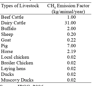
Based on the table 4 can be seen that the value of CH4 emission factor generated from the highest livestock manure produced by the dairy cattle that is equal to 31.00 kg/ animal/year while CH4 emission value of the lowest emission factor produced from poultry group of 0.02 kg/animal/year. The value of emission factor is then multiplied
by the population of livestock and poultry which will be obtained CH4 emission value resulting from cattle and poultry manure.
The highest methane (CH4) emission from livestock manure in 2002 produced by dairy cattle of 10.740 tons; whilst livestock producing the lowest livestock manure emission is horses by 118tons. Such condition is relatively unchanged until 2015, where dairy cows still contribute to the largest methane (CH4) emission. And horse manure is still the lowest contributor of methane emission from livestock manure. If viewed from the average emission of methane produced, dairy cows produce an average methane emission of 13,136 tons per year, while horses produce average methane emission of 102 per year.
When viewed from the value of each livestock emission factor, dairy cow is indeed the highest methane (CH4) emitter Table 4. CH4 Factor Value of Manure
according to Types of Livestock (EFT)
Types of Livestock CH4 Emission Factor (kg/animal/year)
Beef Cattle 1.00
Dairy Cattle 31.00 Buffalo 2.00
Sheep 0.20
Goat 0.22
Pig 7.00
Horse 2.19
Local chicken 0.02
Broiler Chicken 0.02
Laying hens 0.02
Ducks 0.02
Muscovy Ducks 0.02
Source: IPCC, 2006
Table 5. Estimates of Methane Emissions (CH4) from Livestock Manure (ton)
Year Beef Cattle Dairy Cattle Buffalo Goat Sheep Pig Horse 2002 4,295 10,740 1,160 1,533 1,407 1,224 118 2003 4,319 11,212 1,145 1,523 1,435 1,277 117 2004 4,366 10,889 1,188 1,633 1,505 1,570 122
2005 4,415 10,822 931 1,636 1,526 1,637 100
2006 4,419 11,044 926 1,676 1,652 1,511 108
2007 4,707 11,310 922 1,736 1,751 1,343 109
2008 4,869 11,850 917 1,847 1,920 1,402 104
2009 5,751 14,438 907 1,980 1,891 1,307 84
2010 5,988 14,813 915 2,076 1,933 1,359 87
2011 6,669 18,294 725 2,131 2,196 1,507 94
2012 6,951 18,701 720 2,242 2,506 1,621 99
2013 6,439 13,939 596 2,332 2,765 1,755 92
2014 6,786 15,344 623 2,378 3,010 1,562 87
2015 7,029 15,843 616 2,427 3,196 1,529 84
of livestock manure, by 31/kg/animal/ year. It is one of the reasons why dairy cattle contribute the highest methane emissions coming from manure. In terms of the population, beef cattle are more widely bred in Java than the dairy cattle. Nevertheless, the emission factor from beef cattle manure is lower, making the methane emission (CH4) from beef cattle manure become lower than that of dairy cattle.
The methane emission produced by each livestock in Java is growing. This value is in accordance with the increasing number of livestock population in Java, in the period 2002-2015. The methane emission from livestock manure experiencing positive growth is beef cattle (3.65% per year), dairy cows (2.97% per year), goats (3.37% per year), sheep (6.21% Per year), and pigs (1.86% per year). Nevertheless, there are two types of
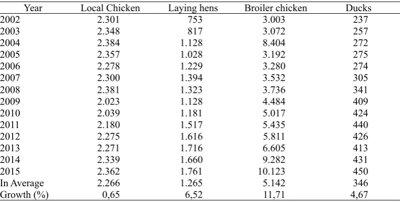
livestock with negative methane emission growth, namely buffalo (-4.68% per year) and horses (-2.46% per year). Such condition is in line with the population of these two which tend to decline each year. Based on the table 6, the methane emission (CH4) yielded by poultry manure in 2002, mostly comes from broiler chicken which is equal to 3.003 tons. In contrast, the poultry producing the least manure methane (CH4) level includes ducks, by 237 tons. Such condition does not change from year to year until 2015, where broiler chicken still have the highest methane emission (CH4) contribution from poultry manure, by 10.123 tons. If viewed from the average value of total methane (CH4) emission from poultry manure, broiler chicken have average methane emission of 5,142 tons per year, whereas ducks have an average methane emission of 346 tons per year.
Table 6. Estimates of Methane Emissions (CH4) from Poultry Manure (ton)
Year Local Chicken Laying hens Broiler chicken Ducks
2002 2.301 753 3.003 237
2003 2.348 817 3.072 257
2004 2.384 1.128 8.404 272
2005 2.357 1.028 3.192 275
2006 2.278 1.229 3.280 274
2007 2.300 1.394 3.532 305
2008 2.381 1.323 3.736 341
2009 2.023 1.128 4.484 409
2010 2.039 1.181 5.017 424
2011 2.180 1.517 5.435 440
2012 2.275 1.616 5.811 426
2013 2.271 1.716 6.605 413
2014 2.339 1.660 9.282 431
2015 2.362 1.761 10.123 450
In Average 2.266 1.265 5.142 346
Growth (%) 0,65 6,52 11,71 4,67
In general, methane emission (CH4) from poultry manure has increased from 2001 to 2015. Furthermore, each type of poultry has grown each year: local chicken by 0.65% per year, laying hens by 6.52 per year, broiler chicken by 11.71% per year, and ducks by 4.67% per year, respectively.
The Analysis of Relationship between
Environmental Degradation (Greenhouse
Gas Emission) and Agricultural GRDP
per Agricultural Labor
In this research, the analysis of relationship between greenhouse gas emission from the agricultural sector and the GRDP per agricultural worker in Java uses The Environmental Kuznets Curve (EKC) model approach. In addition to viewing the relationship, this analysis can be used to reveal whether the agricultural actors have allocated the environmental conservation costs in their agricultural business. In the greenhouse gas emission model, the quadratic function model of GRDP per agricultural
worker is used. The model is:
GHGt=C+ 1GRDP ALt+ 2(GRDP ALt)2+ In the function above, GHGt is the level of greenhouse gas emission from agricultural activity, GRDP AL is GRDP per agricultural worker, and ε is a stochastic disruption. The regression model selection in the panel data is at stage for determining the best estimation method among common effect, fi xed effect and random effect.
Based on the table 7, p-value on chi-square’s cross section is 0.0000<α = 0,05, therefore, H0 is rejected. That is, fi xed effect model is better for use than common effect model.
Based on the table 8, p-value on chi-square’s cross section is 0.0000<α = 0,05, therefore, H0 is rejected. That is, random effect model is better for use than common effect model.
Hausman test is used to fi nd a better model between fi xed effect and random effect models. Based on the table above,
Table 7. Chow Test Analysis Result
Effect Test Statistic d.f. Probability
Cross-section F 796,855263 (4,68) 0,0000
Cross-Section Chi-Sq. 290,142690 4 0,0000
Table 8. Breusch-Pagan Test Analysis Result
Cross-section Test Hyphotesis Time Both
Breusch-Pagan 494,0320
(0,0000)
8,574377 (0,0034)
502,6063 (0,0000)
Table 9. Hausman Test Analysis Result
Test Summary Chi-Sq. Statistic Chi-Sq. d.f. Probability
p-value is 0.8735>α=0.05. That is, H0 fails to be rejected, and therefore, the random effect is better for use.
By the selection of the random effect model, then it is irrelevant to conduct Classic Assumption testing. It is because the random effect model uses the Generalized Least Square (GLS) estimation method. GLS technique is believed to overcome the time series autocorrelation and correlation between observations (cross-sectional) (Lestari and Setyawan, 2017).
The data processing results based on the model suggests the relationship between greenhouse gas emission and GRDP per agricultural worker in Java. The results can be seen in the table 10.
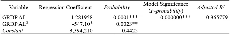
Based on the analysis above, it is known that the quadratic function between greenhouse gas emission and GRDP per agricultural worker in Java has F-probability of 0.0000000 and signifi cant at α = 0.01. These results demonstrate that the EKC model used is appropriate for forecasting. GRDP AL variable and GRDP AL2 are also signifi cant at α= 0.05, and it indicates that there is a relationship between greenhouse
gas emission and GRDP per agricultural worker in Java. Based on the analysis result, the equation of the relationship of both of them is:
GHGt= 3,394,210+1.281958 GRDP ALt -547.10-8 GRDP AL
t 2+
Based on the table, information about the value of regression coeffi cient of GRDP AL and GRDP AL2 variables is earned. The coeffi cient value indicates that the model used has a value of 1> 0 and 2<0. Thereby, that the relationship between greenhouse gas emission and GRDP per agricultural worker in Java forms inverted-U, and it correlates with Environmental Kuznets Curve (EKC) hypothesis. The turning point of the relationship curve between greenhouse gas emission from agricultural activities and GRDP per agricultural worker in Java is known from algebraic calculation on the first derivative equation of quadratic equation obtained in this EKC analysis. The calculation yields a turning point value when GRDP per agricultural worker is Rp. 119,363,000.00. At that level of income, greenhouse gas emission level begins to be Table 10. Estimates of EKC Model of Greenhouse Gas Emission of Agriculture Sector in
Java
Variable Regression Coeffi cient Probability Model Signifi cance
(F-probability) Adjusted-R
2
GRDP AL 1.281958 0.0001*** 0.000000*** 0.365779
GRDP AL2 -547.10-8 0.0023**
Constant 3,394,210 0.4425
equal to GRDP per agricultural worker, where the greater the GRDP value per agricultural worker, the smaller the greenhouse gas emissions incurred - as the agricultural actors begin to compensate some of their income to improve the environment which relates to greenhouse gas emissions. Therefore, there should be an effort to increase the GRDP per worker and start educating agricultural actors to allocate some of their income to improve the environment.
In reality, there are several mitigation technologies as efforts to reduce greenhouse gas emission. The directions for development of adaptive technology are:
a. Low Rice Emission Varieties
Ciherang, cisantana, tukad belian, membramo, Inpari 1, Dodokan, Way Apoburu, dan IR64 includes varieties of greenhouse gas emissions, whereas relatively old varieties such as Cisadane, IR 72, and Ciliwung include high emission verieties (Wihardjaka, 2015).
b. Soil Tillage System
Low methane emissions on land without tillage are suspected as the amount of biomass that is returned to the soil is less than the treatment with perfect soil (Wihardjaka, 2015). c. Regulation of the Water Regime
The intermittent use of irrigation is the most effi cient irrigation management to be able to reduce CH4 gas emissions (Wihardjaka, 2015).
d. Increasing the Composition of Animal Feed Concentrate
Addition of concentrate composition in animal feed followed by the tendency of decreasing of methane gas sourced from digestion. Feeding of 80% concentrate feed can decrease the concentration of methane gas from digestion up to 177 ppm or 28.5% when compared with only grass fed grass (Gustiar et.al., 2014).
e. Low Emission Animal Feed
Selection of feed type greatly affects the size of the methane gas produced by livestock. For example cassava leaves can be used as a means of mitigating methane gas emissions because they contain nitrate salts from Ca, K and Na (Herawati, 2012).
CONCLUSION AND SUGGESTION
Conclusion
a. In overall, greenhouse gas emissions, both CH4 methane emission and (CO2) emissions - resulted from rice cultivation, fertilizer application, livestock enteric fermentation, and livestock & poultry manure - were gradually increasing in the period of 2002-2015.
EKC hypothesis. Furthermore, it was found that it produces turning point value when GRDP per agricultural worker is Rp. 119,363,000,000.00. At that income level, the greenhouse gas emission begins to be equal to GRDP per worker, where the larger the GRDP value per agricultural worker, the smaller the greenhouse gas emission emitted.
Suggestion
The roles of all community elements and government support are needed to implement mitigation technology and agricultural adaptation to deal with impacts of greenhouse gas emission. Some methods of mitigating greenhouse gas emission reduction mainly from the livestock sector are by increasing the concentrate composition in animal feed, ranch maintenance method, the selection of low-emission feed, the management of cattle waste or manure, the processing of feed ingredients, the supplement. In addition, it is expected that the government will make an effort to improve GRDP per agricultural worker through integration policy between sub-sectors of animal husbandry, horticulture, food crops in the agricultural sector so that the inter-sub-sector production process can be more effi cient and able to increase the GRDP per labor of agriculture sector so that the agricultural actors will have more awareness to allocate some of their income to improve the environment.
REFERENCES
Apergis. N. C., Christina. G., Rangan. 2017. Are there Environmental Kuznets Curve for US state-level CO2 emissions?. Renewable and Sustainable Energy Reviews (69): 551-558.
Ariani, M., Setyono, P., Ardiansyah, M.. 2016. Biaya Pengurangan (Marginal Abatement Cost) Emisi Gas Rumah Kaca (GRK) Sektor Pertanian di Kabupaten Grobogan dan Tanjung Jabung Timur. Jurnal Ilmu Lingkungan (14) :39-49.
Azam, M. and K., Abdul Qayyum. 2016. Testing the Environmental Kuzets Curve Hypothesis: A comparative empirical study for low, lower middle, upper middle and high income countries. Renewable and Sustainable Energy Reviews (63): 556-567. Dasgupta, S., Laplante, B., Wang, H., dan
David Wheeler. 2002. Confronting the Enviromental Kuznets Curve . The Journal Of Economic Perspective (1): 147-168.
De Bruyn, S.M., Van den Bergh, J.C., dan J.B. Opschoor 1998. Economic Growth and Emissions: reconsidering the empirical basis of environmental Kuznets curve. Ecological Economics (25): 161-175.
Dinda, S. 2004. Enviromental Kuznets Curve Hypothesis: A Survey. Ecological Economics, (49) :431-455.
Everett, T., Ishwaran., G.P. Ansaloni, dan A. Rubin. 2010. Economic Growth an Environment. Unich Personal RePEc Archive 23585.
Gujarati, D. 2006. Dasar-dasar Ekonometrika. Jilid 2. Jakarta : Erlangga.
Herawati, T. 2012. Refleksi Sosial dari Mitigasi Emisi Gas Rumah Kaca pada Sektor Peternakan di Indonesia. Wartazoa (1): 35-46.
Gustiar, F., Suwignyo, R.A., Suheryanto, Munandar. 2014. Reduksi Gas Metan (CH4) dengan Meningkatkan Komposisi Konstentrat dalam Pakan Ternak Sapi. Jurnal Peternakan Sriwijaya (1): 14-24.
IPCC. 2006. Guidelines for National Green House Gas Inventories, Chapter 10: Emissions from Livestock and Manure Management.
Irham, 2002. Pencemaran Lingkungan dan Aplikasi Kebijakan Pengendaliannya. Jurnal Agroekonomi (1):8-15. Kartikawati R., Susilawati, H.L., Ariani,
M., Setyanto, P. 2011. Teknologi Mitigasi Gas Rumah Kaca dari Lahan Sawah. Jurnal Badan Penelitian dan Pengembangan Pertanian (34):3-8. Lau, L., Choong, C., Eng, Y., 2014.
Investigation of the Environmental Kuznets Curve for carbon emissions in Malaysia: Do foreign direct investment and trade matter?. Energy Policy (68): 490-497.
Lestari, A. dan Setyawan, Y. 2017. Analisis Regresi Data Panel untuk Mengetahui Faktor yang Mempengaruhi Belanja Daerah Provinsi Jawa Tengah. Jurnal Statistika Industri dan Komputasi (1) :1-11.
Sass, R.I. and Cecinore, R.J. 1999. Photosynthate allocations in rice plants: food production or athmosferic methane. http://www.pans.org. [May 24th 2017].
Schutz, H., Seiler, W., and Rennenberg, W. 1990. Soil and land use related souces and sinks of methane (CH4) in context of the global methane budget. In A.F. Bouwman (Ed.). Soils and the Greenhouse Effect., Chichester, New York, Brisbane, Toronto, Singapore : John Wiley and Sons.
Song, T., T. Zheng., dan L. Thong. 2008. An Empirical Test of The Enviromental Kuznets Curve in China: A Panel Cointegration Approach. China Economic Review (199): 381-392. Suarsana, M. and Wahyuni, P.S., 2011. Global
Warming: Ancaman Nyata Sektor Pertanian dan Upaya Mengatasi Kadar CO2 Atmosfer. Jurnal Sains dan Teknologi (11):31-46.
Wang, Y. Han, R. Kobota, J. 2016. Is there an Environmental Kuznets Curve for SO2 emissions? A semi-parametric panel data analysis for China. Renewable and Sustainable Energy Reviews (54):1182-1188.
Widarjono, A. 2009. Ekonometrika, P e n g a n t a r d a n A p l i k a s i n y a. Yogyakarta : Penerbit Ekonisia, Fakultas Ekonomi UII.