Finite Volume Methods
for the One-Dimensional
Shallow Water Equations
Sudi Mungkasi
October 2008
A thesis submitted in partial fulfilment of the requirements for the degree of
Declaration
The work in this thesis is my own except where otherwise stated.
Acknowledgements
I would like to thank AusAID for the Australian Partnership Scholarship so that I could do a Master of Mathematical Sciences at The Australian National Uni-versity in general and complete this thesis in particular.
Special thanks are due to Associate Professor Stephen Roberts for his super-vision on this work. He deserves high honors for carefully guiding me in this research.
I am indebted to many friends or colleagues, but it would take a great deal of space to mention all of them. However, at least I must mention some who have offered substantial support in this research. I would like to thank John Jakeman for the discussions on shallow water equations and on Python programming. Thanks must also go to Hendra Gunawan Harno for several suggestions, and to Gail Craswell, Rhys Michie and Lucille Pedersen for proof-reading the draft of this thesis.
I would also like to express gratitude to my parents and my fianc´ee for their support, encouragement, and unconditional love.
Abstract
This thesis examines the numerical solutions to the one-dimensional shallow wa-ter equations. These solutions are obtained by use of well-balanced finite volume methods, while the well-balanced terms added in the numerical flux computa-tions are based on the steady state of the lake at rest. In addition, the finite volume method being applied is the Kurganov’s central-upwind method, which is a Godunov-type method. Here, the simulations are done to test well-balanced central-upwind finite volume methods with two different sets of reconstructions, namely: stage and momentum, and stage and velocity reconstructions.
The well-balanced central-upwind finite volume methods with stage and mo-mentum reconstructions cannot in general solve the unsteady state problems, such as oscillations in a parabolic canal and dam-break problem in some cases, but these methods work much better to solve steady flow problem than those without well-balanced terms. The performance of the methods with these reconstructions are very dependent on the type of slope limiter being used. These methods using the van Leer slope limiter lead to better results than those using other limiters.
On the other hand, the well-balanced central-upwind finite volume methods with stage and velocity reconstructions are able to capture both unsteady and steady states of water flows. It is an advantage that the performace of the meth-ods are not too dependent on the slope limiter, despite the fact that the methmeth-ods with these reconstructions using superbee limiter yield the smallest error with relatively fast computations. Moreover, the methods with stage and velocity re-constructions result in better performance than those with stage and momentum reconstructions.
Contents
Acknowledgements vii
Abstract ix
Notations and Terminologies xv
1 Introduction 1
1.1 Motivation . . . 1
1.2 Purpose . . . 3
1.3 Outline . . . 3
2 One-Dimensional SWE 5 2.1 Classification of Fluid Flows . . . 5
2.2 Derivation of SWE . . . 7
2.2.1 Conservation of mass . . . 8
2.2.2 Conservation of momentum . . . 11
2.3 Hyperbolic Problems . . . 14
2.3.1 Linear Hyperbolic Equations . . . 17
2.3.2 Domain of Dependence and Range of Influence . . . 19
2.3.3 Riemann Problem . . . 20
2.3.4 Initial-Boundary-Value Problem . . . 22
2.4 Properties of SWE . . . 23
2.4.1 Notion of a Simple Wave . . . 24
2.4.2 Entropy Inequality . . . 26
2.5 Shock Conditions . . . 26
3 Analytical Solutions 31
3.1 Dam-Break Problems . . . 31
3.1.1 Dry-Dam Problem . . . 32
3.1.2 Finite Water Depth Problem . . . 35
3.2 Oscillations in a Parabolic Canal . . . 39
3.3 Steady Flow . . . 43
3.4 Concluding Remarks . . . 45
4 Finite Volume Methods 47 4.1 Approximation of the Quantities and Fluxes . . . 47
4.2 Velocity Stabilization . . . 52
4.3 Slope Limiting . . . 52
4.4 Temporal Discretisation . . . 54
4.5 Boundary Conditions . . . 55
4.6 Properties of Finite Volume Methods . . . 56
4.6.1 Convergence . . . 56
4.6.2 Stability . . . 56
4.6.3 Consistency . . . 57
4.7 Concluding Remarks . . . 58
5 Well-Balanced Finite Volume Methods 59 5.1 Basic Concepts of Well-Balancing . . . 59
5.2 Semi-Discrete First Order Well-Balanced Schemes . . . 62
5.3 Fully Discrete First Order Well-Balanced Schemes . . . 65
5.4 Second Order Well-Balancing . . . 66
5.5 Higher Order Well-Balancing . . . 68
5.6 Quantities Reconstruction . . . 70
5.7 Concluding Remarks . . . 71
6 Stage and Momentum Reconstructions 73 6.1 Test 1: Dam-Break Problems . . . 73
6.1.1 Accuracy . . . 74
6.2 Test 2: Oscillations in a Parabolic Canal . . . 83
6.3 Test 3: Steady Flow . . . 85
6.4 Concluding Remarks . . . 86
7 Stage and Velocity Reconstructions 89 7.1 Test 1: Dam-Break Problems . . . 89
7.1.1 Accuracy . . . 90
7.1.2 Efficiency . . . 92
7.2 Test 2: Oscillations in a Parabolic Canal . . . 93
7.3 Test 3: Steady Flow . . . 96
7.4 Concluding Remarks . . . 96
8 Conclusions 99 A C Tutorial 101 A.1 Preliminaries for C . . . 101
A.2 Types, Operators, and Expressions . . . 104
A.3 Control Flow . . . 106
A.4 Functions and Program Structures . . . 108
A.5 Pointers and Arrays . . . 110
A.6 Structures . . . 112
A.7 Input and Output . . . 113
B C-Python Tutorial 115 B.1 Combining Python with C . . . 117
B.2 Calling C from Python . . . 117
B.3 Example I: Dot Product of Vectors . . . 118
B.4 Example II: Unit Testing . . . 118
B.5 Example III: C-Code for Dot-Product of Vectors . . . 120
Notations and Terminologies
Notations and terminologies which are mostly used are briefly described as fol-lows. The others will be described within the corresponding chapters in this thesis.
Notation
x coordinate in one-dimensional space in the horizontal direction with a unit of metre (m)
t time variable with a unit of second (s)
ρ water density which is assumed to be constant
u(x, t) water velocity at positionx and at time t with a unit of m/s2 h(x, t) water depth which is assumed to vary with the positionx, and
time t with a unit of m
z(x) water bed which is vary only withx with a unit of m
w(x, t) water stage defined as w(x, t) =z(x) +h(x, t) with a unit of m
g gravitational acceleration which is constant and is taken to be 9.81 m/s2
p(x, t) pressure at point (x, t) with a unit of kg/s2
q quantity vector where for one-dimensional shallow water equa-tions q= (h, hu)T
F(q) flux function where for one-dimensional shallow water equa-tions F(q) = (hu, hu2+gh2/2)T
Qn
i numerical approximation to the solutionq, where the subscript
onQdenotes spatial locations, such as theith grid cell, and the superscriptn denotes time leveltn. When Qlacks a temporal
superscript, the current time leveltn is intended.
Terminology
Lagrangian Description of motion where individual particles are observed as a function of time.
Eulerian Description of motion where the flow properties are function of both space and time.
Flow field The region of flow of interest.
Steady flow Flow where quantities do not depend on time, that is
ut =pt=ρt= 0.
List of Figures
2.1 Shallow water flows in one-dimension . . . 9
2.2 The inflow and outflow of the control volume . . . 10
2.3 Pressure in a slope area . . . 11
2.4 Alternative illustration of shallow water flows in one-dimension . . 13
2.5 A typical hyperbolic system of two equations with λ1 < 0 < λ2, (a) shows the domain of dependence of the point (X, T), and (b) shows the range of influence of the point x0. . . 19
2.6 Solution to the Riemann problem for system of two equations in the x, t-plane. . . 22
2.7 Region containing straight characteristics . . . 25
2.8 Discontinuity conditions . . . 27
3.1 Initial water profile of a dam . . . 32
3.2 Water profile of a dry-dam problem at some timet1 >0 . . . 33
3.3 Typical solution of dam-break problem with a finite water depth downstream att =t1 >0. . . 36
3.4 A typical representation of a planar free surface in a parabolic canal. 40 3.5 A typical representation of a steady flow with an obstruction. . . 44
4.1 Updating the cell averagesQn i by fluxes at the cell edges . . . 47
6.1 Well-balanced central-upwind withw-uh reconstructions using 100 cells, first-order spatial discretisation, and first-order time-stepping 75 6.2 Well-balanced central-upwind withw-uh reconstructions using 400
6.3 Well-balanced central-upwind withw-uh reconstructions using 400 cells, second-order spatial discretisation, first-order time-stepping, and minmod limiter . . . 76 6.4 Well-balanced central-upwind withw-uh reconstructions using 400
cells, second-order spatial discretisation, second-order time-stepping, and minmod limiter . . . 76 6.5 Well-balanced central-upwind withw-uh reconstructions using 400
cells, second-order spatial discretisation, first-order time-stepping, and van Leer limiter . . . 78 6.6 Well-balanced central-upwind withw-uh reconstructions using 400
cells, second-order spatial discretisation, second-order time-stepping, and van Leer limiter . . . 78 6.7 Well-balanced central-upwind withw-uh reconstructions using 400
cells, second-order spatial discretisation, second-order time-stepping, and superbee limiter . . . 79 6.8 Well-balanced central-upwind withw-uh reconstructions using 800
cells, second-order spatial discretisation, second-order time-stepping, van Leer limiter and 1 micrometre allowed minimum water depth 79 6.9 Initial water profile in a parabolic canal . . . 84 6.10 Well-balanced central-upwind withw-uh reconstructions using 400
cells, second-order spatial discretisation, second-order time-stepping, and van Leer limiter at t=T /4 . . . 84 6.11 Central-upwind without well-balanced terms using w-uh
recon-structions, 400 cells, order spatial discretisation, second-order time-stepping, and van Leer limiter at t =T /4 . . . 85 6.12 Steady flow using well-balanced central-upwind with w-uh
recon-structions, and 400 cells . . . 87 6.13 Steady flow using well-balanced central-upwind with w-uh
recon-structions, and 1600 cells . . . 87 7.1 Well-balanced central-upwind with w-u reconstructions using 400
cells and van Leer limiter . . . 90 7.2 Well-balanced central-upwind withw-u reconstructions using 3200
7.3 Well-balanced central-upwind with w-u reconstructions using 400 cells and van Leer limiter fort =T /4 . . . 94 7.4 Well-balanced central-upwind with w-u reconstructions using 400
cells and van Leer limiter fort =T /2 . . . 94 7.5 Well-balanced central-upwind with w-u reconstructions using 400
cells and van Leer limiter fort = 3T /4 . . . 95 7.6 Well-balanced central-upwind with w-u reconstructions using 400
cells and van Leer limiter fort =T . . . 95 7.7 Well-balanced central-upwind with w-u reconstructions using 400
cells and superbee limiter . . . 97 7.8 Well-balanced central-upwind with w-u reconstructions using 400
List of Tables
6.1 Absolute errors in water depth, momentum and velocity using 100 cells, second order spatial, second order temporal discretisations and six different limiters . . . 81 6.2 Absolute errors in water depth, momentum and velocity using 400
cells, second order spatial, second order temporal discretisations and six different limiters . . . 81 6.3 Absolute errors in water depth, momentum and velocity using
1,600 cells, second order spatial, second order temporal discretisa-tions and six different limiters . . . 81 6.4 Average time of 10 runs taken to simulate the dam-break problem 82 7.1 Absolute errors in water depth, momentum and velocity using
well-balanced central-upwind with w-u reconstructions using 100 cells and six different slope limiters . . . 91 7.2 Absolute errors in water depth, momentum and velocity using
well-balanced central-upwind with w-u reconstructions using 400 cells and six different slope limiters . . . 91 7.3 Absolute errors in water depth, momentum and velocity using
well-balanced central-upwind withw-u reconstructions using 1600 cells and six different slope limiters . . . 91 7.4 Average time of 10 runs taken to simulate the dam-break problem
with w-u reconstructions . . . 93 7.5 Absolute errors in water depth, momentum and velocity using
well-balanced central-upwind with w-u reconstructions using 400 cells and six different final time . . . 93
Chapter 1
Introduction
This chapter describes the motivation, purpose and outline of this thesis working on Computational Fluid Dynamics. These three aspects are considered as a chronology of why, what, and how this thesis is done.
1.1
Motivation
Computational Fluid Dynamics (CFD) is concerned with the numerical solutions of differential equations which model fluid movement. CFD activity emerged and gained prominence with availability of computers in the early 1960s [15]. Since approximately 1970s there have been commercial computer software packages available, and since that time CFD has become a combination of physics, numer-ical mathematics, and computer sciences [4]. The combination is employed to simulate fluid flows such as gas and water movement.
Shallow Water Equations (SWE) model shallow water flow as the name sug-gests. In general, these equations are according to transport of mass and mo-mentum. These equations form a nonlinear hyperbolic system, and often admit discontinuous solutions even when the initial condition is smooth. They have been widely used for many applications, for example: dam-breaks, tsunami prop-agation, storm surges, solute transport, river flows, and ecological models [27]. Exact solutions to these equations may be investigated by use of characteris-tics methods, but it is often difficult to get those solutions analytically. To deal with this difficulty, numerical methods, such as finite volume methods, have been developed to get the solutions to the SWE.
Finite volume methods are based on the integral form of conservation laws. These methods break the spatial domain into cells and approximate the aver-age of quantity over each cell. In each time step, these values are updated by approximations to the flux through the boundaries of the cells. The main prob-lem of these methods is to determine numerical flux functions which are able to approximate the correct fluxes as close as possible.
Finite volume methods are closely related to finite difference methods, and a finite volume method can often be well viewed as a finite difference approximation to the differential equation. However, since finite volume methods are derived on the basis of the integral form of conservation laws, they admit discontinuities unlike finite difference methods which are derived on the basis of the differential equations. This is why finite volume methods are able to solve the Riemann problem that is a hyperbolic equation together with piecewise constant initial data with a single jump discontinuity.
Many finite volume methods, such as Lax-Friedrichs, Lax-Wendroff, Richt-myer (as also known as Two-Step Lax-Wendroff), and Upwind Godunov Methods, have been developed to get an approximate flux function and have been tested [42]. Jakeman [27] has applied Kurganov’s central-upwind method, which is a finite volume Godunov-type method, with stage and momentum reconstructions for solving the one-dimensional SWE. The scheme in this method was developed by Kurganov, et al. [34, 36], and provide an approximate flux function, which leads to an approximate Riemann solver. It is common that a difficulty arises in the simulation of free surface flows due to the appearance of dry areas which are caused by the initial conditions or as a result of the fluid motion. For ex-ample, there exists oscillations around the interface of wet and dry-regions when Kurganov’s central-upwind method with stage and momentum reconstructions is applied, as can be seen in [27]. Because standard numerical schemes often fail in the presence of wet/dry situations by producing spurious result, modifications in the schemes need to be made [19].
well-balanced.
1.2
Purpose
The purpose of this thesis is to study well-balanced central-upwind finite volume methods for solving one-dimensional SWE. The main idea is to properly combine the central-upwind schemes developed in [36] with the treatment of well-balanced terms in the flux function introduced in [50]. By adding well-balanced terms in the flux function of central-upwind schemes, it is hoped that the resulting methods which are well-balanced can solve the shallow water problems with a better performance.
Combining two tools stated above is by no means an easy task, as many difficulties appear. Values of parameters need to be chosen appropriately during the simulation, and several reconstructions are attempted to know if the methods work. This means that the quantities to be reconstructed have to be properly chosen so as to maintain the well-balanced property, and at the same time to preserve the nonnegativity of the water depth. In addition, schemes satisfying those requirements with inexpensive computation should be taken into account.
1.3
Outline
This thesis is divided into eight chapters. Most of the chapters finish with several concluding remarks of the corresponding topic presented therein.
Chapter 2 presents the basic knowledge related to the SWE. This includes the classification of fluid flow, derivation of the one-dimensional SWE, and properties of the SWE. Hyperbolic problems are also presented since the SWE form a system which admits hyperbolicity.
Chapter 4 describes how finite volume methods are developed. It is started by construction of the approximation of the quantities and fluxes, and followed by presentation on slope limiters to deal with second order spatial discretisation. First and second order temporal discretisation by use of Runge-Kutta methods are also viewed. To complete the presentation, three properties (consisting of convergence, stability and consistency) of finite volume methods as numerical methods are briefly addressed.
The well-balanced finite volume methods are developed in Chapter 5. Even though the well-balanced terms can be constructed from any steady state, the well-balanced methods being discussed in this thesis is limited to those based on the steady state of the lake at rest. It can be seen that the first order well-balanced scheme can be expanded into second order, and then any desired order of well-balanced terms can be obtained by extrapolation.
Simulations of well-balanced finite volume methods are done in Chapter 6 and 7. The finite volume methods being tested are Kurganov’s central-upwind methods. Chapter 6 addresses the tests of well-balanced central-upwind methods with water stage and momentum reconstructions, while Chapter 7 presents the test results of the well-balanced central-upwind methods with stage and velocity reconstructions. All of the numerical methods are tested against the analytical solutions derived in Chapter 3.
Chapter 2
One-Dimensional Shallow Water
Equations
This chapter presents the classification of fluid flows and the derivation of one-dimensional SWE. In addition, topic on hyperbolic equations are viewed as the SWE admit the hyperbolicity property, and properties of the SWE and shock conditions are also presented since it will be considered for the next discussion.
2.1
Classification of Fluid Flows
This section introduces general classification of fluid flows. The classification can be based on the dimension, fluid viscosity, random variation of the particles, and fluid density as described in [57].
a. One-, Two-, and Three-Dimensional Flows
In the Eulerian description, the velocity vector V = (u, v, w)T depends on three
spatial variables and time in general, that is,V=V(x, y, z, t),where the velocity components u, v, and w depend on x,, y, z, and t; this means u = u(x, y, z, t),
v = v(x, y, z, t), and w = w(x, y, z, t). Because the velocity vector depends on three space coordinates, such a flow is a three-dimensional flow. The solutions to three dimensional flows remain three-dimensional even if the flow could be assumed to be steady, that is V=V(x, y, z).
flow, that is a flow in which the velocity vector depends only on two spatial variables. An example is a plane flow (consult [37, 57]) in which the velocity vector depends on two spatial coordinates xand y. Another example is the flow over a wide dam far away from the ends; for this flow, the vertical velocity can be assumed to be zero everywhere, and the horizontal and lateral flows do not depend on z-coordinate but depend only on x and y.
Similarly, aone-dimensional flow is a flow in which the velocity vector depends only on one spatial variable. For example, fluid flows along straight pipes or between parallel plates. For the flow along a straight pipe, the velocity at a point depends only on the the distance between that point to the surface of the pipe. Even if the flow is unsteady, the flow is always one-dimensional.
b. Viscous and Inviscid Flows
A viscous flow is a flow which includes the effects of viscosity, while an inviscid flow is one in which viscous effects do not significantly influence the flow and thus the viscosity of the fluid is neglected. To model an inviscid flow analytically, the viscosity is simply set to be zero so that all viscous effects are zero. To do so, it has to be ensured that the viscous effects are negligibly small.
It has been found from experience that the primary class of flows which can be modeled as inviscid flows isexternal flows, that is, flows which exist exterior to a body. Any viscous effects that may exist are confined to a thin layer, known as a boundary layer which is attached to the boundary. The velocity in a boundary layer is always zero at a fixed wall as a result of viscosity. When the boundary layers are very thin, then they can be ignored so that the flows are assumed to be inviscid.
Viscous flows include a class of internal flows, for example flows in pipes. A substantial amount of energy that must be used to transport oil and gas in pipelines may be lost because of the viscous effects. Such losses are directly caused by the zero velocity at the wall.
c. Laminar and Turbulent Flows
a laminar flow. For a water flow, if it is laminar then a dye injected into the flow will not mix with the neighbouring fluid except by molecular activity. It will retain its identity for a relatively long period of time. If the flow varies irregularly so that flow quantities show random variation then it is called a turbulent flow. When a water flow is turbulent and a dye is injected into it, then the dye will mix immediately. This is caused by random moving of the fluid particles.
d. Incompressible and Compressible Flows
Another classification of fluid flows is that the flows are said to be incompressible or compressible. An incompressible flow exists if the density of each fluid particle remains relatively constant as it moves through the flow field. Otherwise, it is a compressible flow which means that density variations influence the flow.
In general, incompressible flow does not require that the density is constant everywhere. However, if the density of the fluid is known to be constant, then it is clear that the flow is incompressible. It should be noted that constant density is more restrictive than incompressibility. Flows that involve adjacent layers of fresh and salt water, as happens when rivers enter the ocean, are incompressible flows with varying density.
2.2
The derivation of Shallow Water Equations
The SWE are derived based on the fluid motion description. There are two types of fluid motion description, namely Langrangian and Eulerian.
Lagrangian description focuses on individual particles, and its motion is ob-served as a function of time. The position, velocity and acceleration of each particle are listed ass(x0, t),u(x0, t), anda(x0, t), then quantities∗ of interest can
be calculated. Here, the point x0 locates the starting point or the name of each particle. In the Lagrangian description many particles can be followed. However, this becomes difficult as the number of particles in a fluid flow becomes extremely large.
Eulerian description is an alternative to following each fluid particle sepa-rately. This identifies points in space then observes the velocity of particles
ing each point. The rate of change of velocity as the particle pass each point can be observed by ∂u(x, t)/∂x, and the change of velocity with respect to time at each particular point can be observed by∂u(x, t)/∂t. In this Eulerian description of motion, the flow properties (such as velocity) are functions of both space and time.
In the next presentation, equations describing the laws of conservation of mass and momentum are derived for one-dimensional shallow water dynamics problem. Jakeman [27] has adopted Eulerian approach to describe both laws. This thesis takes a different approach to derive the shallow water equations; the conservation of mass is described by Eulerian, but the conservation of momentum is described by Lagrangian.
2.2.1
Conservation of mass
Conservation of mass means that the mass is neither created nor destroyed. This implies that the total mass in the whole system is always the same at any time.
There are several assumptions involved in the derivation of conservation of mass equations. First, the water flow is assumed to be laminar that is the tur-bulent velocity is neglected. Second, the density, ρ, of the water at each point is constant so that the water is incompressible. In addition, it is assumed that the water bed is impermeable because the mass is conserved. Therefore, the mass in any control volume (that is a particular volume or column of water being ob-served) can change only due to the flow acrossing the boundaries of the control volume.
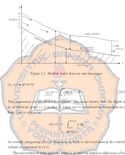
In general, the water flow can be illustrated in Figure 2.1. The notations used in the figure are described as follows:
xrepresents the distance variable along the flow,
t represents the time variable,
z(x) is the fixed water bed,
h(x, t) is the depth of the water at point x and at timet,
w(x, t) =z(x) +h(x, t) is the absolute water level called stage,
u(x, t) denotes the velocity of the water flow at pointx and at time t.
Figure 2.1: Shallow water flows in one-dimension
[x1, x2] is given by
m =
Z x2
x1
ρh(x, t)dx (2.1)
This expression can be obtained as follows. The mass density over the depth ¯ρ
at an arbitrary point (x, t) isρh(x, t) which can be calculated by integration of ρ
from z(x) to w(x, t) as
¯
ρ(x, t) =
Z w(x,t)
z(x)
ρ dy
= ρh(x, t).
As a result, integratingρh(x, t) fromx1 tox2leads to the total mass in the control
volume as expressed in (2.1).
The rate of flow of water past any point (x, t) over the depth is calledmass f lux,
f1 which is given by
f1 = ¯ρ(x, t)u(x, t) (2.2) = ρh(x, t)u(x, t)
acrossing the boundaries of the control volume, it can be found that
Z x2
x1
ρh(x, t+ ∆t)dx=
Z x2
x1
ρh(x, t)dx
+
Z t+∆t
t
ρh(x1, s)u(x1, s)ds−
Z t+∆t
t
ρh(x2, s)u(x2, s)ds (2.3)
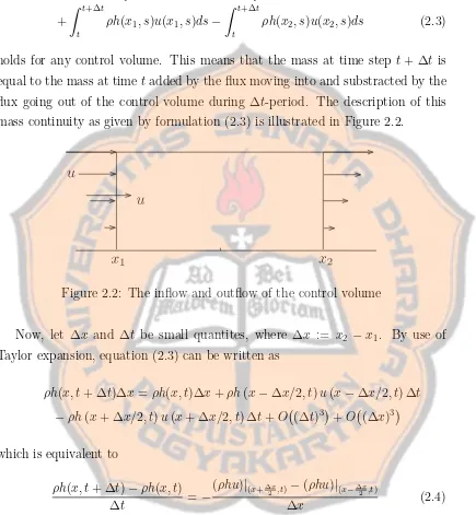
holds for any control volume. This means that the mass at time step t+ ∆t is equal to the mass at timetadded by the flux moving into and substracted by the flux going out of the control volume during ∆t-period. The description of this mass continuity as given by formulation (2.3) is illustrated in Figure 2.2.
Figure 2.2: The inflow and outflow of the control volume
Now, let ∆x and ∆t be small quantites, where ∆x := x2 −x1. By use of Taylor expansion, equation (2.3) can be written as
ρh(x, t+ ∆t)∆x=ρh(x, t)∆x+ρh(x−∆x/2, t)u(x−∆x/2, t) ∆t
−ρh(x+ ∆x/2, t)u(x+ ∆x/2, t) ∆t+O (∆t)3
+O (∆x)3
which is equivalent to
ρh(x, t+ ∆t)−ρh(x, t)
∆t =−
(ρhu)|(x+∆x
2 ,t)−(ρhu)|(x− ∆x
2 ,t)
∆x (2.4)
by neglecting O(∆t3) and O(∆x3) terms. Dividing each term by ρ, and as ∆x
and ∆t approach zero, equation (2.4) becomes
ht+ (uh)x = 0 (2.5)
2.2.2
Conservation of momentum
In this subsection, the conservation of momentum equation using Newton’s second law of motion is presented. The law is that
F = dp
dt
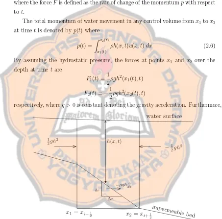
where the forceF is defined as the rate of change of the momentumpwith respect to t.
The total momentum of water movement in any control volume fromx1 tox2
at time t is denoted byp(t) where
p(t) =
Z x2(t)
x1(t)
ρh(x, t)u(x, t) dx (2.6) By assuming the hydrostatic pressure, the forces at points x1 and x2 over the depth at time t are
F1(t) = 1 2ρgh
2(x1(t), t) F2(t) =−1
2ρgh
2(x2(t), t)
respectively, whereg >0 is constant denoting the gravity acceleration. Furthermore,
Figure 2.3: Pressure in a slope area the force over ∆z as shown in Figure 2.3 is
or can be written as
∆F3 =−ρgh(x, t)∆z ∆x∆x
and therefore the force over the bottom of the control volume is
F3 =
Z x2
x1
−ρgh(x, t)zxdx
Hence, the total force over the control volume denoted by F is the sum ofF1, F2
and F3, that is
F = 1
2ρgh
2(x1(t), t)− 1
2ρgh
2(x2(t), t)−
Z x2(t)
x1(t)
ρgh(x, t)dz
dx dx. (2.7)
The first derivative ofp with respect to t is
dp dt =
d dt
Z x2(t)
x1(t)
ρh(x, t)u(x, t) dx
Applying Leibniz’ rule to differentiate this integral yields the relation
dp
dt =
Z x2(t)
x1(t)
∂
∂tρh(x, t)u(x, t) dx
+ρh(x2(t), t)u2(x2(t), t)−ρh(x1(t), t)u2(x1(t), t) (2.8) According to Newton’s second law of motion, the result in equation (2.8) is equal to that in equation (2.7). Hence, for ∆t-period it follows that
Z t+∆t
t
Z x2(t)
x1(t)
(ρhu)t dx dt+
Z t+∆t
t
ρh(x2(t), t)u2(x2(t), t)dt
−
Z t+∆t
t
ρh(x1(t), t)u2(x1(t), t) dt=
Z t+∆t
t
1 2ρgh
2(x1(t), t)dt
Z t+∆t
t
1 2ρgh
2(x2(t), t) dt −
Z t+∆t
t
Z x2(t)
x1(t)
ρgh(x, t)zx dx dt (2.9)
Similar to (2.3), formulation (2.9) can be written as (hu)t+ (hu2+
1 2gh
2)
x =−ghzx
which is called the conservation of momentum equation.
Therefore, the SWE, also known as the Saint-Venant system, can be written as two simultaneous equations
SWE
(
ht+ (hu)x = 0
(hu)t+ (hu2+ 21gh2)x =−ghzx
These two equations are the differential equations of the nonlinear shallow water theory. Once the initial state of the fluid is prescribed, that is once the values of
u and h at the time t = 0 are given, the equations (2.10) yield the subsequent motion.
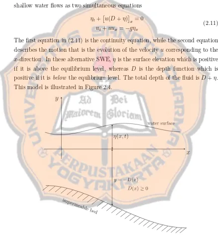
The SWE given by (2.10) above is not the only way to model the shallow water flows. Stoker [66], for instance, models equivalently the one dimensional shallow water flows as two simultaneous equations
ηt+
u(D+η)
x = 0
ut+uux =−gηx
(2.11)
The first equation in (2.11) is the continuity equation, while the second equation describes the motion that is the evolution of the velocity u corresponding to the
x-direction. In these alternative SWE,η is the surface elevation which is positive if it is above the equilibrium level, whereas D is the depth function which is positive if it is below the equlibrium level. The total depth of the fluid is D+η. This model is illustrated in Figure 2.4.
use of these relations, it can be easily shown that (2.10) is equivalent to (2.11) as given in the following theorem.
Theorem 2.1. The systems of equations,
ht+ (hu)x = 0
(hu)t+ (hu2 +21gh2)x =−ghzx
(2.12)
and
ηt+
u(D+η)
x = 0
ut+uux =−gηx
(2.13) are equivalent.
Proof. Substituting D = −z and η = h +z into ηt +
u(D+ η)
x = 0 yield
(h+z)t+ (uh)x = 0. Since zt = 0, the continuity equation,
ht+ (uh)x = 0,
of the SWE is obtained. Now, substituting η =h+z into ut+uux =−gηx and
expanding the result leads to
hut+huux+ghhx =−ghzx,
which can also be written as
[htu] +hut+ [(hu)xu] +huux+ghhx =−ghzx (2.14)
by applying the continuity equation. Furthermore, equation (2.14) can be sim-plified to
(hu)t+
hu2+1 2gh
2
x
=−ghzx.
Hence, the system of equations (2.13) implies (2.12).
By reversing the order of steps above, the system of equations (2.12) implies (2.13). Therefore, both systems of equations are equivalent.
2.3
Hyperbolic Problems
Definition 2.2. A linear system of the form
qt+Aqx= 0,
whereA is a constant coefficient matrix, is calledhyperbolic if the m x mmatrix
A is diagonalizable with real eigenvalues.
There are several special classes of hyperbolic systems according to the prop-erties of matrices A. If A is a symmetric matrix, then A is diagonalizable with real eigenvalues and the system is called symmetric hyperbolic. If A has distinct real eigenvalues, then A is diagonalizable and the system is said to be strictly hyperbolic. If A has real eigenvalues but is not diagonalizable, then the system is called weakly hyperbolic.
There are also other forms of hyperbolic systems. A variable-coefficient linear system of the form
qt+A(x)qx = 0
is hyperbolic at any point x where the coefficient matrix A(x) satisfies the hy-perbolicity condition stated in Definition 2.2. If source term S(x) appears in the system written as
qt+A(x)qx=S(x)
the hyperbolicity still depends on the coefficient matrix, which means that it is hyperbolic at any point where A(x) is diagonalizable with real eigenvalues.
A quasilinear system
qt+A(q, x, t)qx =S(x)
is said to be hyperbolic at a point (q, x, t) if the coefficient matrix A(q, x, t) satisfies the hyperbolicity condition as in Definition 2.2. Hence, the nonlinear conservation law
qt(x, t) +
f q(x, t)
x =S(x), (2.15)
which can also be written in quasilinear form
qt+f′(q)qx=S(x) (2.16)
is hyperbolic if the Jacobian matrixf′(q) satisfies the hyperbolicity condition for
Example 2.3. A simple example of hyperbolic is the scalar, linear, constant coefficient advection equation
qt+ ¯uqx = 0 (2.17)
This equation models the advection of a tracerq along with the fluid, where the fluid velocity ¯u is constant. A tracer here means a substance that is present in very small concentrations whithin the fluid, so that the magnitude of the concentration has essentially no effect on the fluid dynamics.
It is easy to verify that the general solution of (2.17) is any smooth function of the form
q(x, t) = ˜q(x−ut¯ ).
Along any ray in space-time for which x−ut¯ = cst (cst is an abbreviation for constant), the quantity q(x, t) is constant. For example, along the ray X(t) =
x0 + ¯ut, the value of q(X(t), t) is equal to ˜q(x0). The rays X(t) are called the characteristic of the equation. Given the initial data q(x, t0) = ˆq(x), then the particular solution has the form
q(x, t) = ˆq(x−u¯(t−t0))
for t≥t0.
If the space is bounded, a < x < b, then the density of tracer entering the space at the inflow end must also be specified. For example, given that ¯u >0, then two conditions are needed to find the form of the solution. The first condition is a boundary condition at x=a, say
q(a, t) = g0(t) for t≥t0,
and the second condition is the initial condition
q(x, t0) = ˜q(x) for a < x < b.
Considering those conditions, the particular solution is then
q(x, t) =
(
g0(t−(x−a)/u¯) if a < x < a+ ¯u(t−t0) ˆ
q(x−u¯(t−t0)) if a+ ¯u(t−t0)< x < b
Note that when u is not constant and the advection equation is of the form
qt+ [u(x)q]x = 0, the characteristic curves are not straight lines and the solution
Example 2.4. Another example of hyperbolic system, which is also the focus of this thesis, is the SWE (2.10). This system can be expressed by (2.15), where
q = " h uh # = " q1 q2 # , (2.18) f = " uh uh2+gh2/2
#
=
"
q2
(q2)2/q1+gq2 1/2
# , (2.19) and S = " 0
−ghzx
#
=
"
0
−gq1zx
#
. (2.20)
From the explanation above, then the SWE can be written into a quasilinear form (2.16), where the Jacobian matrix f′(q) off is
f′(q) =
"
0 1
−u2+gh 2u
# = " ∂f 1 ∂q1 ∂f1 ∂q2 ∂f2 ∂q1 ∂f2 ∂q2 # . (2.21)
The Jacobian matrix f′(q) has eigenvalues λ1 =u−
p
gh and λ2 =u+
p
gh
with the corresponding eigenvectors
r1 =
"
1
u−√gh
#
and r2 =
"
1
u+√gh
#
.
where g is positive. It is clear that the two eigenvalues are distinct and real if h
is positive. This proves that the SWE (2.10) is strictly hyperbolic whenever h is positive.
2.3.1
Linear Hyperbolic Equations
A linear hyperbolic system of the form
qt+Aqx= 0,
where A is an mxm constant matrix, can be reduced to a set of m decoupled advection equations
where ω = R−1q, A = RΛR−1, and R is the matrix of the right eigenvectors.
This is because A is diagonalisable with real eigenvalues. Suppose that the initial data are given by
q(x,0) = ˆq(x) for − ∞< x <∞,
then ˆω(x) = R−1qˆ(x) satisfies (2.22). The pth equation of (2.22) is the advection
equation
ωp,t+λpωp,x = 0,
which has the solution ωp(x, t) = ωp(x− λpt,0) = ˆωp(x − λpt). All ωp(x, t),
p= 1, . . . , mform ω(x, t). Therefore, the solution to the original problem is
q(x, t) = Rω(x, t) =
m
X
p=1
ωp(x, t)rp, (2.23)
where r1, . . . , rm are the column vectors of the matrix R, as well as the right
eigenvectors of the matrix A
The solution (2.23) can also be written as
q(x, t) =
m
X
p=1
[lpqˆ(x−λpt)]rp, (2.24)
wherel1, l2, . . . , lmare the row vectors ofR−1or the left eigenvectors of the matrix
A. This is because ωp(x, t) =lpq(x, t).
The formula (2.24) can be used even if the initial data ˆq(x) are not smooth, or are even discontinuous, at some points. If the data have a singularity, that is a discontinuity in some derivative at some point x0, then one or more of the
characteristic variables ωp(x,0) will also have a singularity at this point. The
singularities in the initial data will propagate along the characteristics and lead to singularities in the solution q(x, t) at some or all of the points x0 +λpt. On
the other hand, if the initial data are smooth in a neighborhood of all the points ¯
x−λp¯t, then the solution q(x, t) is smooth in a neighborhood of the point (¯x,¯t).
Overall, for a linear system the singularities can only propagate along character-istics.
According to (2.23), the solutionq(x, t) can be viewed as the superposition of
is constant in x for all but one value of p, then the solution to the problem is called simple waves. For example, if ˆωp(x) = ¯ωp for p 6= i, then the initial data
simply propagate with speed λi, that is
q(x, t) = ˆωi(x−λit)ri+
X
p6=i
¯
ωprp = ˆq(x−λit).
2.3.2
Domain of Dependence and Range of Influence
For some fixed point (X, T) in space-time, the solution q(X, T) depends only on the data ˆq atm particular points X−λpT, p= 1, . . . , m. The set of points
D(X, T) ={X−λpT :p= 1, . . . , m},
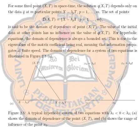
is said to be the domain of dependence of point (X, T). The value of the initial data at other points has no influence on the value of q(X, T). For hyperbolic equations, the domain of dependence is always a bounded set. This is due to the eigenvalues of the matrix coefficient being real, meaning that information propa-gates at finite speed. The domain of dependence for a system of two equations is illustrated in Figure 2.5 (a).
Figure 2.5: A typical hyperbolic system of two equations with λ1 <0 < λ2, (a) shows the domain of dependence of the point (X, T), and (b) shows the range of influence of the point x0.
On the other hand, the data ˆq(x0) will affect the solution along the
charac-teristic rays x0+λpt. The set of points
I(x0, t) ={X+λpt:p= 1, . . . , m}
2.3.3
Riemann Problem
The SWE as in (2.10) can be written in vector form
qt+ [f(q)]x =S (2.25)
where q=q(x, t) is the quantity vector that is the vector of conserved variables,
f represents the flux vector in the x direction and S denotes the source vector. The vectors q, f, and S are given by
q=
"
h hu
#
, f =
"
hu hu2+1
2gh 2
#
, and S =
"
0
−ghzx
#
There is a special type of hyperbolic problem which is called the Riemann problem. This problem is a hyperbolic system together with piecewise constant initial data containing a single jump discontinuity at some point. The initial data is expressed as
q(x, t0) =
(
ql if x < x0
qr if x > x0
To simplify the notation for the Riemann problem, ql andqr can be decomposed
as
ql = m
X
p=1
ωp,lrp and qr= m
X
p=1
ωp,rrp.
Then Riemann data for the pth advection equation are
ˆ
ωp(x) =
(
ωp,l if x < x0
ωp,r if x > x0
Since the discontinuity propagates with speed λp, it is obtained that
ωp(x, t) =
(
ωp,l if x−λpt < x0
ωp,r if x−λpt > x0
By denoting the maximum value of p for which x− λpt > x0 as P(x, t), the
solution q(x, t) can be expressed as
q(x, t) =
P(x,t)
X
p=1
ωp,rrp + m
X
or can be written as
q(x, t) = X
p:λp<(x−x0)/t
ωp,rrp+
X
p:λp>(x−x0)/t
ωp,lrp. (2.26)
Across the pth characteristic the solution jumps with the jump inq given by (ωp,r−ωp,l)rp =αprp,
whereωp,r−ωp,l=αpis a constant. Since the jump is a multiplication of scalar and
rp, this means that the jump inqis an eigenvector of the matrixA. This condition
is called the Rankine-Hugoniot jump condition, derived from the integral form of the conservation law, and seen to hold across any propagating discontinuity.
Solving the Riemann problem for a linear system consists of taking the initial data (ql, qr) and decomposing the jumpqr−ql into eigenvectors of A
qr−ql=α1r1+· · ·+αmrm.
This can be written as a linear system of equations Rα = qr −ql. Therefore,
α = R−1(q
r−ql). The vector α has components αp =lp(qr −ql), where lp’s are
the left eigenvectors of A, so αp =ωp,r−ωp,l.
Sinceαprp is the jump inqacross thepth wave in the solution to the Riemann
problem, this wave can be denoted by
W =αprp.
By use of (2.26), the solution q(x, t) can be written in terms of the waves in two different forms, either
q(x, t) = ql+
X
p:λp<(x−tx0)
Wp
or
q(x, t) =qr−
X
p:λp≥(x−tx0)
Wp.
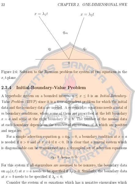
As illustrated by Figure 2.6 in the x, t-plane, for a general Riemann problem for a system of two equations with arbitrary ql and qr, the solution consists of two
discontinuities travelling with speed λ1 and λ2, with a constant state inbetween
denoted by qm. Here,
qm =ω1,rr1+ω2,lr2,
and since ql =ω1,lr1+ω2,lr2 and qr =ω1,rr1+ω2,rr2, it is obtained that
Figure 2.6: Solution to the Riemann problem for system of two equations in the
x, t-plane.
2.3.4
Initial-Boundary-Value Problem
A hyperbolic system on a bounded interval a ≤ x ≤ b is an Initial-Boundary-Value Problem (IBVP) since it is a time-dependent problem for which the initial data and the boundary data are needed. A system ofmequations needs a total of
m boundary conditions, where some of them are prescribed at the left boundary
x = a and some at the right boundary x = b. The number of the needed data at each boundary depends on the number of eigenvalues of A which are positive and negative.
For a simple advection equationqt+ ¯uqx = 0, a boundary condition atx=a
is needed if ¯u > 0 and at x =b if ¯u <0. It is clear that a general system which is diagonalisable can be transformed into a decoupled set of advection equations
ωp,t+λpωp,x = 0.
For this system if all eigenvalues are assumed to be nonzero, the boundary data onωp(x, t) at x=aneeds to be specified if λp >0. Similarly, the boundary data
at x=b needs to be specified if λp <0.
Consider the system of m equations which has n negative eigenvalues which are λ1, λ2, . . . , λn and m−n positive eigenvalues which are λn+1, λn+2, . . . , λm,
where
λ1 ≤λ2 ≤. . .≤λn<0< λn+1, λn+2, . . . , λm.
at x = b to be specified. To impose this type of boundary data, partition the vector ω as
ω=
"
ωI
ωII
#
,
where ωIǫRn and ωIIǫRm−n. Then at the left boundary, the components of ωII
must be specified whileωI are outflow variables. This can be done by writingωII
in terms ofωI, such as a linear boundary condition of the form
ωII(a, t) =B1ωI(a, t) +g1(t),
where B1ǫR(m−n)xn and g1ǫRm−n. If B1 = 0, then the inflow variables are given without effect of the outflow. However, there is often a reflection of outgoing waves through a physical boundary, and this requires a nonzero matrix B1.
2.4
Properties of the Shallow Water Equations
To solve the SWE, understanding its properties will be useful. This section ex-plores several of the SWE properties and assumes that the water bed topography is flat, unless stated explicitly. Since the topography is flat, the SWE is considered homogeneous.
By using a gas dynamics analogy, new quantities
¯
ρ=ρh and ¯p=
Z w
z
p dy
can be introduced where ¯ρand ¯pare the density-like and pressure-like respectively. In view of the hydrostatic pressure law, the last equation can be expreesed as
¯
p= gρ¯
2
2ρ .
Here, the depth of water is in place of density in a gas. By recalling the sound speed or the propagation speed which is given by c=p
¯
p′(¯ρ) as in acoustics, this
quantity is then given by
c=
r
gρ¯
ρ =
p
gh.
By applying the method of characteristic there are two sets of characteristic curves, C1 and C2, which are the solution curves of the ordinary differential equations
(
C1 : dxdt =u+c, and
C2 : dxdt =u−c . (2.27)
The functions u +c and u− c are the eigenvalues of the coefficient matrix as shown in Example 2.4. The relations
(
u+ 2c=k1 = cst along a curveC1 and,
u−2c=k2 = cst along a curveC2. (2.28)
hold, and are known as Riemann invariants. In addition, the constantsk1 and k2
are different on different curves and the two families of characteristics given by (2.27) are distinct since c6= 0 for h 6= 0. Furthermore, the system of equations (2.27) together with (2.28) are equivalent to the homogeneous SWE.
2.4.1
Notion of a Simple Wave
Suppose that the initial water state is uniform, that is at time t= 0 the particle velocity and the sound speed are u = u0 = cst and c = c0 = √gh = cst
respec-tively. Now suppose that a disturbance is initiated at the origin x = 0 so that either u or c changes with the time. This means a disturbance at one point in the water propagates into water of constant depth and uniform velocity. Under these conditions, it can be proved that one of the two families of characteristics given by ordinary differential equations (2.27) consists entirely of straight lines along each of which u and c are constant, and then the corresponding motion is called simple wave. To make it clear, this statement is written in the following theorem.
Theorem 2.5. One of the two families of characteristics given by ordinary dif-ferential equations
( dx
dt =u+c, and dx
dt =u−c
(2.29)
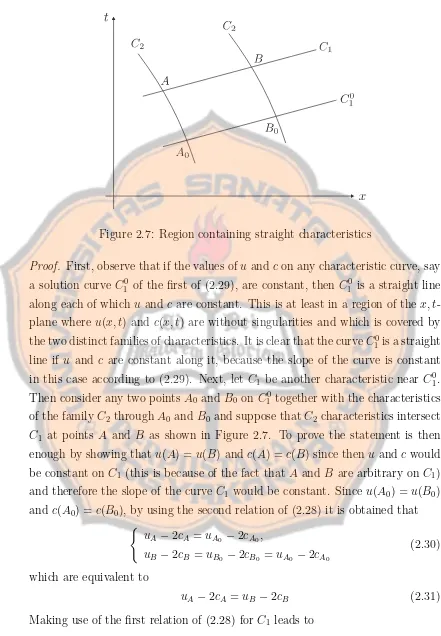
Figure 2.7: Region containing straight characteristics
Proof. First, observe that if the values ofuandcon any characteristic curve, say a solution curve C0
1 of the first of (2.29), are constant, thenC10 is a straight line
along each of which u and c are constant. This is at least in a region of the x, t -plane where u(x, t) and c(x, t) are without singularities and which is covered by the two distinct families of characteristics. It is clear that the curveC0
1 is a straight
line if u and c are constant along it, because the slope of the curve is constant in this case according to (2.29). Next, let C1 be another characteristic near C0
1.
Then consider any two pointsA0 and B0 onC0
1 together with the characteristics
of the familyC2 throughA0 andB0 and suppose thatC2 characteristics intersect
C1 at points A and B as shown in Figure 2.7. To prove the statement is then enough by showing that u(A) =u(B) andc(A) = c(B) since then uand cwould be constant on C1 (this is because of the fact that Aand B are arbitrary on C1)
and therefore the slope of the curve C1 would be constant. Since u(A0) =u(B0) and c(A0) =c(B0), by using the second relation of (2.28) it is obtained that
(
uA−2cA=uA0 −2cA0,
uB−2cB =uB0 −2cB0 =uA0 −2cA0
(2.30)
which are equivalent to
uA−2cA=uB−2cB (2.31)
Making use of the first relation of (2.28) for C1 leads to
It is clear that (2.31) and (2.32) can only be satisfied if uA = uB and cA = cB.
This completes the proof.
2.4.2
Entropy Inequality
The SWE model (2.10) above has a hyperbolic type and admits an entropy in-equality related to the physical energy. The derivation of the entropy inin-equality can be found in [6], and is given by
˜
ηt(q, z) + ˜Gx(q, z)≤0
where
˜
η(q, z) = η(q) +ghz, G˜(q, z) = G(q) +ghzu,
and
η(q) =hu2/2 + g 2h
2, G(q) = (hu2/2 +gh2)u.
2.5
Shock Conditions
By expressing the SWE into quasilinear form and assuming the solution is smooth, it can be shown that there are two families of characteristics producing a curvilin-ear coordinate system overx, t-plane. However, that is often not the case because the solution may not be smooth in some problems.
In theory, when two or more characteristics of the same family intersect, a discontinuity known as shock will occur. In this case, to investigate the solutions, the integral form of the conservation law must be applied. Given s is the shock propagating speed, it can be shown that across any shock the Rankine-Hugoniot condition
s(qr−ql) =f(qr)−f(ql)
must be satisfied. However, the Rankine-Hugoniot condition does not guarantee a unique solution. To determine whether a weak solution is indeed the physically correct solution, applying the Lax entropy condition is needed. This condition is satisfied if the characteristics converge such that
for the 1-shock and the 2-shock respectively. Here λ1 = u− √
gh and λ2 = u+√gh are the eigenvalues of the Jacobian matrix f′(q) which are often called
the characteristic speeds.
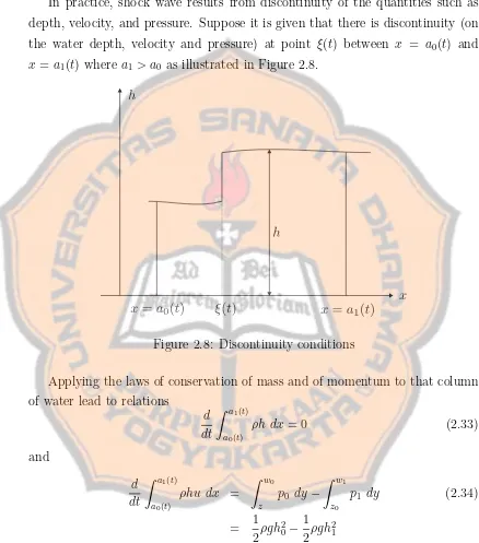
In practice, shock wave results from discontinuity of the quantities such as depth, velocity, and pressure. Suppose it is given that there is discontinuity (on the water depth, velocity and pressure) at point ξ(t) between x = a0(t) and
x=a1(t) where a1 > a0 as illustrated in Figure 2.8.
Figure 2.8: Discontinuity conditions
Applying the laws of conservation of mass and of momentum to that column of water lead to relations
d dt
Z a1(t)
a0(t)
ρh dx= 0 (2.33)
and
d dt
Z a1(t)
a0(t)
ρhu dx =
Z w0
z
p0 dy−
Z w1
z0
p1 dy (2.34)
= 1 2ρgh
2 0−
1 2ρgh
2 1
The integrals in these relations have the form
I =
Z a1(t)
a0(t)
ψ(x, t) dx
where ψ(x, t) is discontinuous atx=ξ(t). Applying Leibniz’ rule to differentiate this integral yields the relation
dI
dt =
d dt
Z ξ(t)
a0(t)
ψ dx+ d
dt
Z a1(t)
ξ(t)
ψ dx (2.35)
=
Z a1(t)
a0(t)
∂ψ
∂t dx+ψ(ξ−, t) ˙ξ(t)−ψ(a0(t), t)u0
+ψ(a1(t), t)u1−ψ(ξ+, t) ˙ξt
Here, u0 = ˙a0(t) = d
dta0(t) and u1 = ˙a1(t) = d
dta1(t) are the velocities at the ends
of the column, ˙ξ is the velocity of the discontinuity, andψ(ξ−, t) andψ(ξ+, t) are
the limit value of ψ to the left and to the right of x =ξ. By taking the limit in which the length of the column tends to zero in such away that the discontinuity remains inside the column, the integral on the right-hand side of (2.35) tends to zero, and it is obtained that
lim
l→0 dI
dt =ψ1v1−ψ0v0. (2.36)
Here, l =a1−a0 is the length of the column,v1 =u1−ξ˙ andv0 =u0−ξ˙ are the flow velocities relative to the moving discontinuity, and ψ1 and ψ0 refer to the limit values of ψ to the right and to the left of the discontinuity respectively.
According to the presentation on the previous paragraph, using (2.36) for the limit cases which arise from (2.33) and (2.34), it is obtained that
ρh1v1−ρh0v0 = 0 (2.37)
and
ρh1u1v1−ρh0u0v0 = 1 2ρgh 2 0− 1 2ρgh 2
1. (2.38)
Equations (2.37) and (2.38) can also be written as ¯
ρ1v1 = ¯ρ0v0 (2.39)
and
¯
where ¯ρ=ρh and ¯p= 1 2ρgh
2 = g
2ρρ¯
2. A discontinuity satisfying (2.39) and (2.40)
is referred to as ashock wave or simply as ashock or as abore, or if it is stationary as a hydraulic jump.
Another way of expressing the shock conditions (2.39) and (2.40) is
(
¯
ρ1v1 = ¯ρ0v0 =m,
m(v1−v0) = ¯p0−p1,¯ (2.41) where m represents the mass flux across the shock front.
Consider a special case where u0 = 0 which means the water is at rest on one side of of the shock. Since mv1 = ¯ρ0v0v1 and mv0 = ¯ρ1v1v0, the second of the shock conditions (2.41) can be expressed as
v1v0 = p0¯ −p1¯ ¯
ρ0−ρ¯1
. (2.42)
Since u0 = 0, it is clear that v0 = −ξ˙ and v1 = u1 −ξ˙ so that (2.42) takes the form
−ξ˙(u1 −ξ˙) = g
2ρ(¯ρ0+ ¯ρ1) (2.43)
by using the relation ¯p= 2gρρ¯2 and ρ=ρ0 =ρ1. Similarly, since u0 = 0, the first
shock condition now takes the form ¯
ρ1(u1−ξ˙) =−ρ0¯ξ.˙ (2.44) Furthermore, ifu1 is eliminated, the second shock condition (2.43) can be written as
˙
ξ2 = gρ1¯ 2ρ 1 +
¯
ρ1
¯
ρ0
; (2.45)
or if ¯ρ0 is eliminated, it can also be written as
−ξ˙(u1 −ξ˙) = gρ1¯
2ρ 1−
u1−ξ˙
˙
ξ
(2.46) Therefore, (2.44) together with either (2.43), (2.45), or (2.46) are alternative ways of expressing the shock conditions when u0 = 0.
2.6
Concluding Remarks
Chapter 3
Analytical Solutions to the
Shallow Water Equations
This chapter considers three specific types of problems relating to the SWE and presents their analytical solutions. These three problems are: dam-break prob-lems, oscillations in a parabolic canal, and steady flow over a parabolic obstruc-tion.
3.1
Dam-Break Problems
This section presents the determination of the flow which results from a sudden destruction of a dam. The considered problem is the SWE (2.10) with a flat-bottom topography (flat water bed), that is zx = 0, such that
ht+ (hu)x = 0,
(hu)t+ (hu2+ 12gh2)x = 0
)
(3.1)
The construction of analytical expressions of this problem can be found in [66]. The solutions to dam-break problems have been presented by several authors (see [27, 75]).
The classification of dam-break problems can be based on the initial position and the initial depth of the downstream side. If the downstream of a dam is on the right side then the problem is called a rightward dam-break because the water will move in a rightward direction after the dam is broken, otherwise it is a leftward dam-break. If the initial depth of the downstream side is zero then it
is known as dry-dam, otherwise it is known as a finite water depth problem.
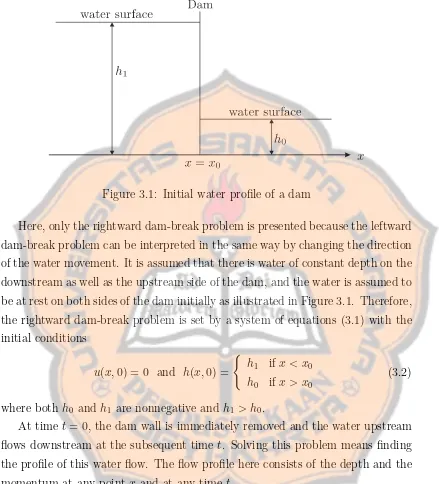
Figure 3.1: Initial water profile of a dam
Here, only the rightward dam-break problem is presented because the leftward dam-break problem can be interpreted in the same way by changing the direction of the water movement. It is assumed that there is water of constant depth on the downstream as well as the upstream side of the dam, and the water is assumed to be at rest on both sides of the dam initially as illustrated in Figure 3.1. Therefore, the rightward dam-break problem is set by a system of equations (3.1) with the initial conditions
u(x,0) = 0 and h(x,0) =
(
h1 if x < x0
h0 if x > x0 (3.2)
where both h0 and h1 are nonnegative and h1 > h0.
At time t= 0, the dam wall is immediately removed and the water upstream flows downstream at the subsequent time t. Solving this problem means finding the profile of this water flow. The flow profile here consists of the depth and the momentum at any point x and at any time t.
3.1.1
Dry-Dam Problem
Consider a dry-dam problem where the initial conditions are given by (3.2) with
x0 = 0 and h0 = 0.
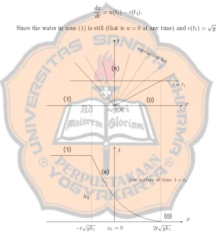
The typical solution of a dam-break problem on to a dry bed at some time
that three different regions in the fluid at t = t1 are considered. The zone (0)
is the zone of dry-bed downstream which is terminated by the tip of a parabolic surface or rarefaction zone (R); the rarefaction zone (R) connects the dry-bed zone (0) with the zone of undisturbed water upstream (1).
The point on the surface which connects zone (1) and (R) at t=t1 satisfies dx
dt =u(t1)−c(t1).
Since the water in zone (1) is still (that isu= 0 at any time) and c(t1) = √
gh1
Figure 3.2: Water profile of a dry-dam problem at some time t1 >0
it is obtained that
dx
dt =−
p
Therefore, the motion of that point satisfies x=−t√gh1.
Consider the rarefaction fan in zone (R). Each of the characteristics satisfies
dx
dt =u(t1)−c(t1). (3.3)
Along each of the characteristics in zone (R), according to (2.28) the Riemann invariant u−2cis constant. Therefore,
u(t1)−2c(t1) =u1−2c1 (3.4) in which u1 andc1 are the known values ofuandcin the zone (1). Hence, as one sees from (3.3) and (3.4) the slope of any straight characteristics can be given by either of the two forms:
dx dt =
3
2u(t1)−c1, or
dx
dt = 2c1−3c.
(3.5) The slope in this zone cannot be negative, otherwise the water depth will be negative. Preserving the water depth to be nonnegative requires thatu(t1)≤2c1. In other words, the zone (R) is terminated by a point which moves on the line
x= 2t√gh1. In zone (R), the slopes of the characteristics are
dx dt =
x t.
According to (3.5), dx/dt= 3
2u(t1)−c1, so that x
t =
3
2u−c1, which is equivalent to
u= 2 3
p
gh1+ x
t
.
In addition, from the second relation of (3.5), it can be obtained the value of c
within zone (R) that
c= 2 3c1−
x
3t
This last equation leads to h= 94g √gh1− x
2t
2
.
Therefore, the free surface water profile and velocity at any time t1 > 0 for the dry-dam problem with zero initial velocity are given by
h(x) =
h1 if x≤ −t√gh1
hR= 94g(√gh1− 2xt)2 if −t√gh1 < x≤2t√gh1
0 if x≥2t√gh1
and
u(x) =
0 if x≤ −t√gh1
uR = 23(√gh1+ xt) if−t√gh1 < x≤2t√gh1
0 if x≥2t√gh1
(3.7)
The quantities at the position of the dam are interesting. At x = 0 it is obvious that the depth of the water at the site of the dam is always 49h1 which is constant. The velocity of the water at this point is also constant and has the value u = 2
3 √
gh1. Thus, the volume rate of discharge of water at the original location of the dam is constant and has the value ofhu= 8h
27 √
gh1. It can also be
observed that the water depth, velocity and discharge at everyxwill converge to these values as t→ ∞.
Note that the solutions (3.6) and (3.7) are only for a dry-bed problem with horizontal bottom topography. For an ideal fluid flow, these solution may be extended using a technique called the method of superposition [12, 11] so that for a mild, constant slope, the solutions of the SWE are given by
h(x) =
h1 if−1> t√x
gh1
hR= h91
2 + b0t
2
qg
h1 −
x t√gh1
2
if−1≤ x
t√gh1 ≤2 +
b0t
2
q g
h1
0 ift√x
gh1 >2 +
b0t
2
q
g h1 and
u(x) =
0 if−1> t√x
gh1
uR = 2
√
gh1
3
1 +b0tqhg1 + t√x
gh1
if−1≤ x
t√gh1 ≤2 +
b0t
2
qg
h1
0 ift√x
gh1 >2 +
b0t
2
q
g h1
where zx =b0 is the bed slope which is positive for downwardslope, and x-axes
is the bed (note that x-axes is not the horizontal axes).
3.1.2
Finite Water Depth Problem
Figure 3.3: Typical solution of dam-break problem with a finite water depth downstream at t=t1 >0.
When the dam is immediately removed, as shown in Figure 3.3, the spatial domain is separated into four regions which are from left to right: first still region or region (1) where the depth is the same as initial water depth h1, parabolic surface region or region (3) with depth h3, constant region or region (2) with
depth h2, and second still region or region (0) where the depth is the same as initial water depthh0. Region (2) is connected to the undisturbed water upstream (region (1)) by a rarefaction fan with a parabolic surface. This parabolic surface expands, while a shock moving to the right forms between the constant region (2) and the second still region (0).
The point at which region (1) and region (3) meet is determined by the char-acteristic
while the point separating region (3) and region (2) is determined by
x= (u2−c2)t,
and the position of the shock moving at speed ˙ξ is given by x = ˙ξt. Here,
ci = √ghi, where i = 1,2,3, are the wave propagation speed in water of depth
hi.
In region (3), the characteristic curves are determined by
dx dt =
x
t =u3−c3.
Along each of the characteristic in this region, the Riemann invariants u+ 2c
is constant. Therefore, on the left extreme of the rarefaction fan it is true that
u+ 2c= 2c1, and along the rarefaction fan it is also true thatu+ 2c=u3+ 2c3. Following this,
2c1 =u3+ 2c3. (3.8)
Substituting c3 =u3−x/t to (3.8) results in u3 = 23(c1+x/t) or
u3 = 2 3(c1+
x
t). (3.9)
Furthermore, substituting (3.9) to (3.8) leads to c3 = 13(2c1−x/t) or
h3 =
4 9g
p
gh1− x
2t
2
.
At the interface between region (2) and (0), it is convenient to write the shock conditions for the passage from state (0) to the state (2) in the form
−ξ˙(u2−ξ˙) = 1
2(c
2
0+c22), (3.10)
and
c22(u2−ξ˙) =−c20ξ,˙ (3.11) which are the same as (2.43) and (2.44) with c2
i = ghi in place of gρ¯i/ρ. To get
the expression of u2 , the variable c2
2 needs to be eliminated from (3.10) by use
of (3.11), and then the resulting quadratic needs to be solved for u2 and to be simplified so that it can be written
u2 = ˙ξ− c 2 0
4 ˙ξ
1 +
q
1 + 8( ˙ξ/c0)2
This yields
u2 = ˙ξ− gh0
4 ˙ξ
1 +
s
1 + 8 ˙ξ
2
gh0
. (3.13)
In the expression (3.12), the plus sign before the radical was taken in order that
u2−ξ˙and−ξ˙have the same sign; and it can be observed that only positive values of ˙ξand u2 need to be determined throughout the entire discussion since the side of (0) is the front side of the shock and the positive x-direction is taken to the right. Now, to get the expression ofc2, the variableu2 needs to be eliminate from (3.10) by use of (3.11), and then the result can be expressed in the form
c2 c0 = 1 2 q
1 + 8( ˙ξ/c0)2− 1
2
1/2
. (3.14)
This leads to
h2 = h0
2
s
1 + 8 ˙ξ2
gh0 −1
.
Equations (3.13) and (3.14) provide expression of the velocityu2 and the wave speed c2 in the constant region (2) behind the shock as functions of the shock
speed ˙ξand the wave propagation speedc0in the undisturbed region (0). Consider the rarefaction fan in region (3). Along each of the characteristics x/t = u−c
in this region, the Riemann invariant u+ 2c is constant. Therefore, on the left extreme and on the right extreme of the rarefaction fan
u+ 2c= 2c1 and u+ 2c=u2 + 2c2
respectively. According to these two relations, it is clear that 2c1 =u2+2c2. Since
the form of u2 and c2 have been determined in (3.13) and (3.14), it is obtained that
c1 = ξ˙ 2 −
c2 0
8 ˙ξ
"
1 +
s
1 + 8 ˙ξ
2 c0 # + " c2 0 2 s
1 + 8 ˙ξ
2
c0 − c2
0
2
#
which can be rewritten as
˙
ξ= 2c1+ c
2 0
4 ˙ξ
"
1 +
s
1 + 8 ˙ξ
2 c2 0 # − "
2c20
s
1 + 8 ˙ξ
2
c2 0 −
2c20
#1/2
. (3.15)
a compact form
h(x) =
h1 if x≤ −t
√ gh1 h3 = 94g(√gh1− x
2t)2 if −t
√
gh1 < x≤t(u2−√gh2)
h2 = h0
2
q
1 + 8 ˙ghξ2 0 −1
if t(u2−√gh2)< x < tξ˙
h0 if x≥tξ˙
and
u(x) =