gensen
•Takesanexample-basedapproach,withclearandauthoritativeexplanations •IntroducesbothSQLandthequerytoolsusedtoexecuteSQLstatements •Showshowtocreatetables,populatethemwithdata,andthenquerythatdata
•Createdatabasetablesanddefinetheirrelationships •Adddatatoyourtables.Thenchangeanddeletethatdata •Writedatabasequeriesthatgenerateaccurateresults
•AvoidcommontrapsandpitfallsinwritingSQLqueries,especiallyfromnulls •Reaptheperformanceandexpressivenessofanalyticandwindowfunctions •MakeuseofOracleDatabase’ssupportforobjecttypes
For your convenience Apress has placed some of the front
matter material after the index. Please use the Bookmarks
Contents at a Glance
About the Authors ...
xvii
About the Technical Reviewer ...
xix
Acknowledgments ...
xxi
Introduction ...
xxiii
Chapter 1: Relational Database Systems and Oracle
■
...
1
Chapter 2: Introduction to SQL and SQL Developer
■
...
23
Chapter 3: Data Definition, Part I
■
...
59
Chapter 4: Retrieval: The Basics
■
...
69
Chapter 5: Retrieval: Functions
■
...
.101
Chapter 6: Data Manipulation
■
...
129
Chapter 7: Data Definition, Part II
■
...
147
Chapter 8: Retrieval: Multiple Tables and Aggregation
■
...
.177
Chapter 9: Retrieval: Some Advanced Features
■
...
213
Chapter 10: Views
■
...
.245
Chapter 11: SQL*Plus Basics and Scripting
■
...
267
Chapter 12: Object-Relational Features
■
...
.323
Appendix A: The Seven Case Tables
■
...
341
Appendix B: Answers to the Exercises
■
...
.351
Introduction
This book was born from a translation of a book originally written by Lex de Haan in Dutch. That book was first published in 1993, and went through several revisions in its native Dutch before Lex decided to produce an English version. Apress published that English version in 2005 under the title “Mastering Oracle SQL and SQL*Plus”. The book has since earned respect as an excellent, accurate, and concise tutorial on Oracle’s implementation of SQL.
While SQL is a fairly stable language, there have been changes to Oracle’s implementation of it over the years. The book you are holding now is a revision of Lex’s original, English-language work. The book has been revised to cover new developments in Oracle SQL since 2005, especially those in Oracle Database 11g Release 1 and Release 2, and Oracle Database 12c Release 1. The book has also been given the title “Beginning Oracle SQL”. The new title better positions the book in Apress’s line, better reflects the content, fits better with branding and marketing efforts, and marks the book as a foundational title that Apress intends to continue revising and publishing in the long term.
About this Book
This is not a book about advanced SQL. It is not a book about the Oracle optimizer and diagnostic tools. And it is not a book about relational calculus, predicate logic, or set theory. This book is a SQL primer. It is meant to help you learn Oracle SQL by yourself. It is ideal for self-study, but it can also be used as a guide for SQL workshops and instructor-led classroom training.
This is a practical book; therefore, you need access to an Oracle environment for hands-on exercises. All the software that you need to install Oracle Database on either Windows or Linux for learning purposes is available free of charge from the Oracle Technology Network (OTN). Begin your journey with a visit to the OTN website at:
http://www.oracle.com/technology/index.html
From the OTN home page, you can navigate to product information, to documentation and manual sets, and to free downloads that you can install on your own PC for learning purposes.
This edition of the book is current with Oracle Database 12c Release 1. However, Oracle SQL has been reasonably stable over the years. All the examples should also run under 11g Release 2. And most will still run under Oracle Database 10g, under Oracle Database 9i, and even under Oracle Database 8i, if you’re running software that old. Of course, as you go further back in release-time, you will find more syntax that is not supported in each successively older release. Oracle Corporation does tend to add a few new SQL features with each new release of their database product.
Oracle Corporation has shown great respect for SQL standards over the past decade. We agree with supporting standards, and we follow the ANSI/ISO standard SQL syntax as much as possible in this book. Only in cases of useful, Oracle-specific SQL extensions do we deviate from the international standard. Therefore, most SQL examples given in this book are probably also valid for other database management system (DBMS) implementations supporting the SQL language.
■ INTRODUCTION
Listing I-1. A SQL SELECT Statement
SELECT 'Hello world!' FROM dual;
One difference between this edition and its predecessor is that we omit the “SQL>” prompt from many of our examples. That prompt comes from SQL*Plus, the command-line interface that old-guard database administrators and developers have used for years. We now omit SQL*Plus prompts from all examples that are not specific to SQL*Plus. We do that out of respect for the growing use of graphical interfaces such as Oracle SQL Developer.
This book does not intend (nor pretend) to be complete; the SQL language is too voluminous and the Oracle environment is much too complex. Oracle’s SQL reference manual, named the Oracle Database SQL Language Reference, comes in at just over 1800 pages for the Oracle Database 12c Release 1 edition. Moreover, the current ISO SQL standard documentation has grown to a size that is simply not feasible anymore to print on paper.
The main objective of this book is the combination of usability and affordability. The official Oracle
documentation offers detailed information in case you need it. Therefore, it is a good idea to have the Oracle manuals available while working through the examples and exercises in this book. The Oracle documentation is available online from the OTN website mentioned earlier in this introduction. You can access that documentation in HTML form, or you can download PDF copies of selected manuals.
The focus of this book is using SQL for data retrieval. Data definition and data manipulation are covered in less detail. Security, authorization, and database administration are mentioned only for the sake of completeness in the “Overview of SQL” section of Chapter 2.
Throughout the book, we use a case consisting of seven tables. These seven tables contain information about employees, departments, and courses. As Chris Date, a well-known guru in the professional database world, said during one of his seminars, “There are only three databases: employees and departments, orders and line items, and suppliers and shipments.”
The amount of data (i.e., the cardinality) in the case tables is deliberately kept low. This enables you to check the results of your SQL commands manually, which is nice while you’re learning to master the SQL language. In general, checking your results manually is impossible in real information systems due to the volume of data in such systems.
It is not the data volume or query response time that matters in this book. What’s important is the database structure complexity and SQL statement correctness. After all, it does no good for a statement to be fast, or to perform well, if all it does in the end is produce incorrect results. Accuracy first! That’s true in many aspects of life, including in SQL.
About the Chapters of this Book
Chapter 1 provides a concise introduction to the theoretical background of information systems and some popular database terminology, and then continues with a global overview of the Oracle software and an introduction to the seven case tables. It is an important, foundational chapter that will help you get the most from the rest of the book.
Chapter 2 starts with a high-level overview of the SQL language. SQL Developer is then introduced. It is a tool for testing and executing SQL. It is a nice, fairly intuitive graphical user interface, and it is a tool that has gained much ground and momentum with developers. Free download and documentation can be found here:
http://www.oracle.com/technetwork/developer-tools/sql-developer/downloads/index.html
Retrieval is also spread over multiple chapters—four chapters, to be precise. Chapter 4 focuses on the SELECT,
WHERE, and ORDER BY clauses of the SELECT statement. The most important SQL functions are covered in Chapter 5, which also covers null values and subqueries. In Chapter 8, we start accessing multiple tables at the same time (joining tables) and aggregating query results; in other words, the FROM, the GROUP BY, and the HAVING clauses get our attention in that chapter. To finish the coverage of data retrieval with SQL, Chapter 9 revisits subqueries to show some more advanced subquery constructs. That chapter also introduces windows and analytic functions, the row limiting clause, hierarchical queries, and flashback features.
Chapter 6 discusses data manipulation with SQL. The commands INSERT, UPDATE, DELETE, and MERGE are introduced. This chapter also pays attention to some topics related to data manipulation: transaction processing, read consistency, and locking.
In Chapter 7, we revisit data definition, to drill down into constraints, indexes, sequences, and performance. Synonyms are explained in the same chapter. Chapters 8 and 9 continue coverage of data retrieval with SQL.
Chapter 10 introduces views. What are views, when should you use them, and what are their restrictions? This chapter explores the possibilities of data manipulation via views, discusses views and performance, and introduces materialized views.
Chapter 11 is about automation and introduces the reader to the SQL*Plus tool. SQL statements can be long, and sometimes you want to execute several in succession. Chapter 11 shows you how to develop automated scripts that you can run via SQL*Plus. SQL*Plus is a command-line tool that you can use to send a SQL statement to the database and get results back. Many database administrators use SQL*Plus routinely, and you can rely upon it to be present in any Oracle Database installation. Many, many Oracle databases are kept alive and healthy by automated SQL*Plus scripts written by savvy database administrators.
Oracle is an object-relational database management system. Since Oracle Database 8, many object-oriented features have been added to the SQL language. As an introduction to these features, Chapter 12 provides a high-level overview of user-defined datatypes, arrays, nested tables, and multiset operators.
Finally, the book ends with two appendixes. Appendix A at the end of this book provides a detailed look into the example tables used in this book’s examples. Appendix B gives the exercise solutions.
About the Case Tables
CHAPTER 1
Relational Database Systems
and Oracle
The focus of this book is writing SQL in Oracle, which is a relational database management system. This first chapter provides a brief introduction to relational database systems in general, followed by an introduction to the Oracle software environment. The main objective of this chapter is to help you find your way in the relational database jungle and to get acquainted with the most important database terminology.
The first three sections discuss the main reasons for automating information systems using databases, what needs to be done to design and build relational database systems, and the various components of a relational database management system. The following sections go into more depth about the theoretical foundation of relational database management systems.
This chapter also gives a brief overview of the Oracle software environment: the components of such an environment, the characteristics of the components, and what you can do with those components.
The last section of this chapter introduces seven sample tables, which are used in the examples and exercises throughout this book to help you develop your SQL skills. In order to be able to formulate and execute the correct SQL statements, you’ll need to understand the structures and relationships of these tables.
This chapter does not cover object-relational database features. In Chapter 12 you will find information about Oracle features in that area.
1.1 Information Needs and Information Systems
Organizations have business objectives. In order to realize those business objectives, many decisions must be made on a daily basis. Typically, a lot of information is needed to make the right decisions; however, this information is not always available in the appropriate format. Therefore, organizations need formal systems that will allow them to produce the required information, in the right format, at the right time. Such systems are called information systems. An information system is a simplified reflection (a model) of the real world within the organization.
Information systems don’t necessarily need to be automated—the data might reside in card files, cabinets, or other physical storage mechanisms. This data can be converted into the desired information format using certain procedures or actions. In general, there are two main reasons to automate information systems:
• Complexity: The data structures or the data processing procedures become too complicated. • Volume: The volume of the data to be administered becomes too large.
The main advantages of using database technology are as follows:
• Accessibility: Ad hoc data-retrieval functionality, data-entry and data-reporting facilities, and concurrency handling in a multiuser environment
• Availability: Recovery facilities in case of system crashes and human errors • Security: Data access control, privileges, and auditing
• Manageability: Utilities to efficiently manage large volumes of data
When specifying or modeling information needs, it is a good idea to maintain a clear separation between
information and application. In other words, we separate the following two aspects:
• What: The information content needed. This is the logical level and it represents the
information.
• How: The desired format of the information, the way that the results can be derived from the data stored in the information system, the minimum performance requirements, and so on. This is the physical level and it represents the application.
Database systems such as Oracle enable information system users and designers/developers to maintain this separation between the “what” and the “how” aspects, allowing users of such systems to concentrate more on the first aspect and less on the second. This is because database system implementations are based on the relational model. The relational model is explained later in this chapter, in Sections 1.4 through 1.7.
1.2 Database Design
One of the problems with using traditional third-generation programming languages (such as COBOL, Pascal, Fortran, and C) is the ongoing maintenance of existing code, because these languages don’t separate the “what” and the “how” aspects of information needs. That’s why programmers using those languages sometimes spend more than 75% of their precious time on maintenance of existing programs, leaving little time for them to build new programs.
When using database technology, organizations usually need many database applications to process the data residing in the database. These database applications are typically developed using fourth- or fifth-generation application development environments, which significantly enhance productivity by enabling users to develop database applications faster while producing applications with lower maintenance costs. However, in order to be successful using these fourth- and fifth-generation application development tools, developers must start thinking about the structure of their data first.
It is very important to spend enough time on designing the data model before you start coding your applications. Data model mistakes discovered in a later stage, when the system is already in production, are very difficult and expensive to fix.
Entities and Attributes
In a database, we store facts about certain objects. In database jargon, such objects are commonly referred to as
entities. For each entity, we are typically interested in a set of observable and relevant properties, commonly referred to as attributes.
When designing a data model for your information system, you begin with two questions:
1. Which entities are relevant for the information system?
CHAPTER 1 ■ RELATIONAL DATABASE SYSTEMS AND ORACLE
For example, consider a company in the information technology training business. Examples of relevant entities for the information system of this company could be course attendee, classroom, instructor, registration, confirmation, invoice, course, and so on. An example of a partial list of relevant attributes for the entity
COURSE_ATTENDEE could be the following: Registration number
For the COURSE entity, the attribute list might include attribute items such as: Title
■
There are many different terminology conventions for entities and attributes, such as
objects
,
object types
,
types
,
object occurrences
, and so on. The terminology itself is not important, but once you have made a choice, you
should use it consistently.
Generic vs. Specific
The difference between generic versus specific is very important in database design. For example, common words in natural languages such as book and course have both generic and specific meanings. In spoken language, the precise meaning of these words is normally obvious from the context in which they are used.
When designing data models, you must be very careful about the distinction between generic and specific meanings of the same word. For example, a course has a title and a duration (generic), while a specific course offering has a location, a start date, a certain number of attendees, and an instructor. A specific book on the shelf might have your name and purchase date on the inside cover page, and it might be full of your personal annotations. On the other hand, a generic book has a title, an author, a publisher, and an ISBN code. This means that you should be careful when using words like course and book for database entities, because they could be confusing and suggest the wrong meaning.
Redundancy
There are two types of data: base data and derivable data. Base data is data that cannot be derived in any way from other data residing in the information system. It is crucial that base data is stored in the database. Derivable data can be deduced (for example, with a formula) from other data. For example, if we store both the age and the date of birth of each course attendee in our database, these two attributes are mutually derivable—assuming that the current date is available at any moment.
Actually, every question issued against a database results in derived data. In other words, it is both undesirable and not reasonable to store all derivable data in an information system. Storage of derivable data is referred to as
redundancy. Another way of defining redundancy is storage of the same data more than once.
Sometimes, it makes sense to store redundant data in a database; for example, in cases where response time is crucial and in cases where repeated computation or derivation of the desired data would be too time-consuming. But typically, storage of redundant data in a database should be avoided. First of all, it is a waste of storage capacity. However, that’s not the biggest problem, since terabytes of disk capacity can be bought for relatively low prices these days. The challenge with redundant data storage lies in its ongoing maintenance.
With redundant data in your database, it is difficult to process data manipulation correctly under all circumstances. In case something goes wrong, you could end up with an information system containing internal contradictions. In other words, you could have inconsistent data. Therefore, redundancy in an information system may result in ongoing consistency problems.
When considering the storage of redundant data in an information system, it is important to distinguish two types of information systems:
Online transaction processing (OLTP) systems, which typically have continuous data changes •
and high volume
Decision support systems (DDS; often referred to as data warehouses), which are mainly, or •
even exclusively, used for data retrieval and reporting, and are loaded or refreshed at certain frequencies with data from OLTP systems
In DSS systems, it is common practice to store a lot of redundant data to improve system response times. Retrieval of stored data is typically faster than data derivation, and the risk of inconsistency, although present for load and update of data, is less likely because most DSS systems are often read-only from the end user’s perspective.
Consistency, Integrity, and Integrity Constraints
Obviously, consistency is a first requirement for any information system, ensuring that you can retrieve reliable information from that system. In other words, you don’t want any contradictions in your information system.
For example, suppose we derive the following information from our training business information system: Attendee 6749 was born on February 13, 2093.
•
The same attendee 6749 appears to have gender Z. •
There is another, different attendee with the same number 6749. •
We see a course registration for attendee 8462, but this number does not appear in the •
administration records where we maintain a list of all attendees.
In none of the above four cases is the consistency at stake; the information system is unambiguous in its statements. Nevertheless, there is something wrong because these statements do not conform to common sense.
CHAPTER 1 ■ RELATIONAL DATABASE SYSTEMS AND ORACLE
3. Every course attendee (or person, in general) has a unique number.
4. We have registration information only for existing attendees—that is, attendees known to the information system.
These rules concerning database contents are called constraints. You should translate all your business rules into formal integrity constraints. The third example (in the list above)—a unique number for each person—is a primary key constraint, and it implements entity integrity. The fourth example—information for only persons known to the system—is a foreign key constraint, implementing referential integrity. We will revisit these concepts later in this chapter, in Section 1.5.
Constraints are often classified based on the lowest level at which they can be checked. The following are four constraint types, each illustrated with an example:
• Attribute constraints: Checks attributes; for example, “Gender must be M or F or O.” • Row constraints: Checks at the row level; for example, “For salesmen, commission is a
mandatory attribute.”
• Table constraints: Checks at the table level; for example, “Each employee has a unique e-mail address.”
• Database constraints: Checks at the database level; for example, “Each employee works for an existing department.”
In Chapter 7, we’ll revisit integrity constraints to see how you can formally specify them in the SQL language. At the beginning of this section, you learned that information needs can be formalized by identifying which entities are relevant for the information system and deciding which attributes are relevant for each entity. Now we can add a third step to the information analysis list of steps you’ve learned thus far to produce a formal data model:
1. Which entities are relevant for the information system?
2. Which attributes are relevant for each entity?
3. Which integrity constraints should be enforced by the system?
Data Modeling Approach, Methods, and Techniques
The job of designing appropriate data models is not a sinecure and is typically a task for IT specialists. And although end users are not what you may think of as the parties responsible for assisting in data model design, it is almost impossible to design data models without the active participation of the future end users of the system. End users usually have the most expertise in their professional area, and IT specialists use this expertise to their advantage when designing data models. Additionally, a seasoned IT specialist ensures that the end users are also involved in the final system acceptance tests.
Over the years, many methods have been developed to support the system development process itself, to generate system documentation, to communicate with project participants, and to manage projects to control time and costs. Traditional methods typically show a strict phasing of the development process and a description of what needs to be done in which order. That’s why these methods are also referred to as waterfall methods. Roughly formulated, these methods distinguish the following four phases in the system development process:
1. Analysis: Describing the information needs and determining the information system boundaries
2. Logical design: Getting answers to the three questions about entities, attributes, and constraints, the concepts presented in the previous section
Within the development methods, you can use various techniques to support your activities. For example, you can use diagram techniques to represent data models graphically. Some well-known examples of such diagram techniques are Entity Relationship Modeling (ERM) and Unified Modeling Language (UML). In the last section of this chapter, which introduces the sample tables used throughout this book, you will see an ERM diagram that corresponds with those tables.
Another example of a well-known technique is normalization, which allows you to remove redundancy from a database design by following some strict rules.
Prototyping is also a quite popular technique. Using prototyping, you produce “quick and dirty” pieces of functionality to simulate parts of a system, with the intention of evoking reactions from the end users. This might result in time-savings during the analysis phase of the development process, and more importantly, better-quality results, thus increasing the probability of system acceptance at the end of the development process.
Rapid application development (RAD) is another well-known term associated with data modeling. Instead of the waterfall approach described earlier, you employ an iterative approach.
Some methods and techniques are supported by corresponding computer programs, which are referred to as computer-aided systems engineering (CASE) tools. Various vendors offer complete and integral support for system development, from analysis to system generation (Oracle’s SQL Developer Data Modeler is one example), while others provide basic support for database design even though their products are general-purpose drawing tools (Microsoft Visio is an example).
Semantics
If you want to use information systems correctly, you must be aware of the semantics (the meaning of things) of the underlying data model. A careful choice for table names and column names is a good starting point, followed by applying those names as consistently as possible. For example, the attribute “address” can have many different meanings: home address, work address, mailing address, and so on. The meaning of attributes that might lead to this type of confusion can be stored explicitly in an additional semantic explanation to the data model. Although such a semantic explanation is not part of the formal data model itself, you can store it in a data dictionary—a term explained in Section 1.3.
Information Systems Terms Review
CHAPTER 1 ■ RELATIONAL DATABASE SYSTEMS AND ORACLE
1.3 Database Management Systems
The preceding two sections defined the formal concept of an information system. You learned that if an organization decides to automate an information system, it typically uses some database technology. The term database can be defined as follows:
Definition
■
A
database
is a set of data, which is needed to derive the desired information from an information system
and maintained by a separate software program.
This separate software program is called the database management system (DBMS). There are many types of database management systems available, varying in terms of the following characteristics:
Price •
Ability to implement complex information systems •
Supported hardware environment •
Flexibility for application developers •
Flexibility for end users •
Ability to set up connections with other programs •
Speed (performance) •
Ongoing operational costs •
User-friendliness •
Ability to guarantee data consistency •
Ability to support concurrent access by multiple users •
DBMS Components
A DBMS has many components, including a kernel, data dictionary, query language, and tools.
Kernel
Data Dictionary
Another important task of the DBMS is the maintenance of a data dictionary, containing all data about the database (the metadata). Here are some examples of information maintained in a data dictionary:
Overview of all entities and attributes in the database •
Constraints (integrity) •
Access rights to the data •
Additional semantic explanations •
Database user authorization data •
Query Languages
Each DBMS vendor supports one or more languages to allow access to the data stored in the database. These languages are commonly referred to as query languages. SQL, the language this book is all about, has been the de facto market standard for many years.
OTHER QUERY LANGUAGES, REALLY?
SQL is such a common query language that very few realize that there were ever any others. In fact, few even
comprehend the concept that there exist query languages other than SQL. But there are others. Oracle Rdb
supports SQL, but Rdb also supports a language called Relational Database Operator (RDO). (Yes, you’ve heard it
here: there was an RDO long before Microsoft took up that abbreviation). RDO is a language developed by Digital
Equipment Corporation (DEC) for use in their own database management system. Oracle bought that system
and continues to support the use of RDO to this day.The Ingres database, once a competitor to Oracle, also had
its own query language. Ingres originally supported a language known as Quel. That language did not compete
well with SQL, and Ingres Corporation was eventually forced to build SQL support into their product.Today, SQL
is the dominant database access language. All mainstream relational databases claim to support it. And yet, no
two databases support it in quite the same way. Instead of completely different languages with dissimilar names,
today we have “variations” that we refer to as Oracle SQL, Microsoft SQL, DB2 SQL, and so forth. The world really
hasn’t changed much.
DBMS Tools
Most DBMS vendors supply many secondary programs around their DBMS software. The authors of this book refer to all these programs with the generic term tools. These tools allow users to perform tasks such as the following:
Generate reports •
Build standard data-entry and data-retrieval screens •
Process database data in text documents or in spreadsheets •
CHAPTER 1 ■ RELATIONAL DATABASE SYSTEMS AND ORACLE
Database Applications
Database applications are application programs that use an underlying database to store their data. Examples of such database applications are screen- and menu-driven data-entry programs, spreadsheets, report generators, and so on.
Database applications are often developed using development tools from the DBMS vendor. In fact, most of these development tools can be considered to be database applications themselves, because they typically use the database not only to store regular data, but also to store their application specifications. For example, consider tools such as Oracle JDeveloper, Oracle SQL Developer, and Oracle Application Express. With these examples we are entering the relational world, which is introduced in Section 1.4.
DBMS Terms Review
In this section, the following terms were introduced: Database
The theoretical foundation for a relational database management system (RDBMS) was laid out in 1970 by Ted Codd in his famous article “A Relational Model of Data for Large Shared Data Banks” (Codd, 1970). He derived his revolutionary ideas from classical components of mathematics: set theory, relational calculus, and relational algebra.
About ten years after Ted Codd published his article, around 1980, the first RDBMS systems aiming to translate Ted Codd’s ideas into real products became commercially available. Among the first pioneering RDBMS vendors were Oracle and Ingres, followed a few years later by IBM with SQL/DS and DB2.
We won’t go into great detail about this formal foundation for relational databases, but we do need to review the basics in order to explain the term relational. The essence of Ted Codd’s ideas was two main requirements:
Clearly distinguish the logical task (the
• what) from the physical task (the how) both while designing, developing, and using databases.
Make sure that an RDBMS implementation fully takes care of the physical task, so the system •
users need to worry only about executing the logical task.
These ideas, regardless of how evident they seem to be nowadays, were quite revolutionary in the early 1970s. Most DBMS implementations in those days did not separate the logical and physical tasks at all; did not have a solid theoretical foundation of any kind; and offered their users many surprises, ad hoc solutions, and exceptions. Ted Codd’s article started a revolution and radically changed the way people think about databases.
1.5 Relational Data Structures
This section introduces the most important relational data structures and concepts: Tables, columns, and rows
•
The information principle •
Datatypes •
Keys •
Missing information and null values •
Tables, Columns, and Rows
The central concept in relational data structures is the table or relation (from which the relational model derives its name). A table is defined as a set of rows, or tuples (pronounced like couples). The rows of a table share the same set of attributes; a row consists of a set of (attribute name; attribute value) pairs. All data in a relational database is represented as column values within table rows.
In summary, the basic relational data structures are as follows: A database, which is a set of tables
•
A table, which is a set of rows •
A row, which is a set of column values •
The definition of a row is a little imprecise. A row is not just a set of column values. A more precise definition would be as follows:
A
• row is a set of ordered pairs, where each ordered pair consists of an attribute name with an associated attribute value.
For example, the following is a formal and precise way to represent a row from the DEPARTMENTS table:
{(deptno;40),(dname;HR),(location;Boston),(mgr;7839)}
This row represents department 40: the HR department in Boston, managed by employee 7839. It would become irritating to represent rows like this; therefore, this book will use less formal notations as much as possible. After all, the concept of tables, rows, and columns is rather intuitive.
CHAPTER 1 ■ RELATIONAL DATABASE SYSTEMS AND ORACLE
The Information Principle
The only way you can associate data in a relational database is by comparing column values. This principle, known as the information principle, is applied very strictly, and it is at the heart of the term relational.
An important property of relational datasets is the fact that the order of their elements is meaningless. Therefore, the order of the rows in any relational table is meaningless, too, and the order of columns is also meaningless.
Because this is both very fundamental and important, let’s rephrase this in another way: in a relational
database, there are no pointers to represent relationships. For example, the fact that an employee works for a specific department can be derived only from the two corresponding tables by comparing column values in, for example, the two department number columns. In other words, for every retrieval command, you must explicitly specify which columns must be compared. As a consequence, the flexibility to formulate ad hoc queries in a relational database has no limits. The flip side of the coin is the risk of (mental) errors and the problem of the correctness of your results. Nearly every SQL query will return a result (as long as you don’t make syntax errors), but determining whether it is really the answer to the question you had in mind is up to you.
Datatypes
One of the tasks during data modeling is to decide which values are allowed for each attribute. You could allow only numbers in a certain column, or allow only dates or text. You can impose additional restrictions, such as by allowing only positive integers or text of a certain maximum length.
A set of allowed attribute values is sometimes referred to as a domain. Another common term is datatype (or simply type). Each attribute is defined to be of a certain type. This can be a standard (built-in) type or a user-defined type.
Keys
Each relational table must have at least one candidate key. A candidate key consists of an attribute (or attribute combination) that uniquely identifies each row in that table, with one additional important property: as soon as you remove any attribute from this candidate key attribute combination, the property of unique identification is gone. In other words, a table cannot contain two rows with the same candidate key values at any time and still maintain row uniqueness.
For example, the attribute combination course CODE and BEGINDATE is a candidate key for a table containing information about course offerings. If you remove the BEGINDATE attribute, the remaining course CODE attribute is not a candidate key anymore; otherwise, you could offer courses only once. If you remove the course CODE attribute, the remaining BEGINDATE attribute is not a candidate key anymore; otherwise, you would never be able to schedule two different courses to start on the same day.
In case a table has multiple candidate keys, it is normal practice to select one of them to become the primary key. All components (attributes) of a primary key are mandatory; you must specify attribute values for all of them. Primary keys enforce a very important table constraint: entity integrity.
Sometimes, the set of candidate keys doesn’t offer a convenient primary key. In such cases, you may choose a
surrogate key by adding a meaningless attribute with the sole purpose of being the primary key.
Note
■
The use of surrogate keys comes with advantages and disadvantages, as well as fierce debates between
database experts. The intent of this section is to explain the terminology, without offering an opinion on the use of
surrogate keys.
A relational table can also have one or more foreign keys. Foreign key constraints are subset requirements; the foreign key values must always be a subset of a corresponding set of primary key values. Some typical examples of foreign key constraints are that an employee can work for only an existing department and can report to only an existing manager. Foreign keys implement referential integrity in a relational database.
Missing Information and Null Values
A relational DBMS is supposed to treat missing information in a systematic and context-insensitive manner. If a value is missing for a specific attribute of a row, it is not always possible to decide whether a certain condition evaluates to
true or false. Missing information is represented by null values in the relational world.
The term null value is actually misleading, because it does not represent a value; it represents the fact that a value is missing. For example, null marker would be more appropriate. However, null value is the term most commonly used, so this book uses that terminology. Figure 1-2 shows how null values appear in a partial listing of the EMPLOYEES table.
Figure 1-2. Nulls represent missing values
Null values imply the need for a three-valued logic, such as implemented (more or less) in the SQL language. The third logical value is unknown.
Note
CHAPTER 1 ■ RELATIONAL DATABASE SYSTEMS AND ORACLE
Constraint Checking
Although most RDBMS vendors support integrity constraint checking in the database these days (Oracle implemented this feature a number of years ago), it is sometimes also desirable to implement constraint checking in client-side database applications. Suppose you have a network between a client-side data-entry application and the database, and the network connection is a bottleneck. In that case, client-side constraint checking probably results in much better response times, because there is no need to access the database each time to check the constraints. Code-generating tools typically allow you to specify whether constraints should be enforced at the database side, the client side, or both sides.
Caution
■
If you implement certain constraints in your client-side applications only, you risk database users bypassing
the corresponding constraint checks by using alternative ways to connect to the database.
Predicates and Propositions
To finish this section about relational data structures, there is another interesting way to look at tables and rows in a relational database from a completely different angle, as introduced by Hugh Darwen. This approach is more advanced than the other topics addressed in this chapter, so you might want to revisit this section later.
You can associate each relational table with a table predicate and all rows of a table with corresponding propositions. Predicates are logical expressions, typically containing free variables, which evaluate to true or false. For example, this is a predicate:
There is a course with title
• T and duration D, price P, frequency F, and a maximum number of attendees M.
If we replace the five variables in this predicate (T, D, P, F, and M) with actual values, the result is a proposition. In logic, a proposition is a predicate without free variables; in other words, a proposition is always true or false. This means that you can consider the rows of a relational table as the set of all propositions that evaluate to true.
Relational Data Structure Terms Review
In this section, the following terms were introduced: Tables (or relations)
Integrity checking at the database level •
Missing information, null values, and three-valued logic •
Predicates and propositions •
1.6 Relational Operators
type you provided as input (numbers). For example, for integers, addition is closed. Add any two integers, and you get another integer. Try it—you can’t find two integers that add up to a noninteger. However, division over the integers is
not closed; for example, 1 divided by 2 is not an integer. Closure is a nice operator property, because it allows you to (re)use the operator results as input for a next operator’s operation.
In a database environment, you need operators to derive information from the data stored in the database. In an RDBMS environment, all operators should operate at a high logical level. This means, among other things, that they should
not operate on individual rows, but rather on tables, and that the results of these operations should be tables, as well. Because tables are defined as sets of rows, relational operators should operate on sets. That’s why some operators from the classical set theory—such as the union, the difference, and the intersection—also show up as relational operators. See Figure 1-3 for an illustration of these three set operators.
Figure 1-3. The three most common set operators
Along with these generic operators from set theory that can be applied to any sets, there are some additional relational operators specifically meant to operate on tables. You can define as many relational operators as you like, but, in general, most of these operators can be reduced to (or built with) a limited number of basic relational operators. The most common relational operators are the following:
• Restriction: This operator results in a subset of the rows of the input table, based on a specified restriction condition. This operator is also referred to as selection.
• Projection: This operator results in a table with fewer columns, based on a specified set of attributes you want to see in the result. In other words, the result is a vertical subset of the input table.
• Union: This operator merges the rows of two input tables into a single output table; the result contains all rows that occur in at least one of the input tables.
• Intersection: This operator also accepts two input tables; the result consists of all rows that occur in both input tables.
CHAPTER 1 ■ RELATIONAL DATABASE SYSTEMS AND ORACLE
• (Cartesian) product: From two input tables, all possible combinations are generated by concatenating a row from the first table with a row from the second table.
• (Natural) Join: From two input tables, one result table is produced. The rows in the result consist of all combinations of a row from the first table with a row from the second table, provided both rows have identical values for the common attributes.
Note
■
The natural join is an example of an operator that is not strictly necessary, because the effect of this operator
can also be achieved by applying the combination of a Cartesian product, followed by a restriction (to check for identical
values on the common attributes), and then followed by a projection to remove the duplicate columns.
1.7 How Relational Is My DBMS?
The term relational is used (and abused) by many DBMS vendors these days. If you want to determine whether these vendors speak the truth, you are faced with the problem that relational is a theoretical concept. There is no simple litmus test to check whether or not a DBMS is relational. Actually, to be honest, there are no pure relational DBMS implementations. That’s why it is better to investigate the relational degree of a certain DBMS implementation.
This problem was identified by Ted Codd, too; that’s why he published 12 rules (actually, there are 13 rules, if you count rule zero, as well) for relational DBMS systems in 1986. Since then, these rules have been an important yardstick for RDBMS vendors. Without going into too much detail, Codd’s rules are listed here, with brief explanations:
1. Rule Zero: For any DBMS that claims to be relational, that system must be able to manage databases entirely through its relational capabilities.
2. The Information Rule: All information in a relational database is represented explicitly at the logical level and in exactly one way: by values in tables.
3. Guaranteed Access Rule: All data stored in a relational database is guaranteed to be logically accessible by resorting to a combination of a table name, primary key value, and column name.
4. Systematic Treatment of Missing Information: Null values (distinct from the empty string, blanks, and zero) are supported for representing missing information and inapplicable information in a systematic way, independent of the datatype.
5. Dynamic Online Catalog: The database description is represented at the logical level in the same way as ordinary data so that authorized users can apply the same relational language to its interrogation as they apply to the regular data.
6. Comprehensive Data Sublanguage: There must be at least support for one language whose statements are expressible by some well-defined syntax and are comprehensive in supporting all of the following: data definition, view definition, data manipulation, integrity constraints, authorization, and transaction boundaries handling.
7. Updatable Views: All views that are theoretically updatable are also updatable by the system.
9. Physical Data Independence: Application programs remain logically unimpaired whenever any changes are made in either storage representations or access methods.
10. Logical Data Independence: Application programs remain logically unimpaired when information-preserving changes that theoretically permit unimpairment are made to the base tables.
11. Integrity Independence: Integrity constraints must be definable in the relational data sublanguage and storable in the catalog, not in the application programs.
12. Distribution Independence: Application programs remain logically unimpaired when data distribution is first introduced or when data is redistributed.
13. The NonsubversionRule: If a relational system also supports a low-level language, that low-level language cannot be used to subvert or bypass the integrity rules and constraints expressed in the higher-level language.
Rule 6: Comprehensive Data Sublanguage refers to transactions. Without going into too much detail here, a transaction is defined as a number of changes that should be treated by the DBMS as a single unit of work; a transaction should always succeed or fail completely. For further reading, please refer to Oracle Insights: Tales of the Oak Table by Dave Ensor (Apress, 2004), especially Chapter 1.
1.8 The Oracle Software Environment
Oracle Corporation has its headquarters in Redwood Shores, California. It was founded in 1977, and it was (in 1979) the first vendor to offer a commercial RDBMS.
The Oracle software environment is available for many different platforms, ranging from personal computers (PCs) to large mainframes and massive parallel processing (MPP) systems. This is one of the unique selling points of Oracle: it guarantees a high degree of independence from hardware vendors, as well as various system growth scenarios, without losing the benefits of earlier investments, and it offers extensive transport and communication possibilities in heterogeneous environments.
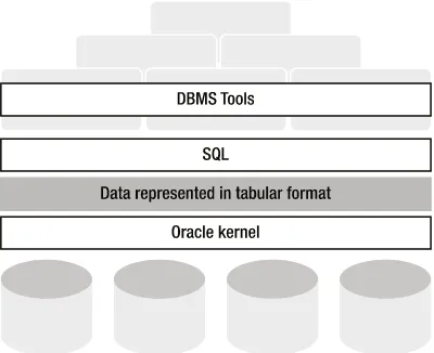
The Oracle software environment has many components and bundling options. The core component is the DBMS itself: the kernel. The kernel has many important tasks, such as handling all physical data transport between memory and external storage, managing concurrency, and providing transaction isolation. Moreover, the kernel ensures that all stored data is represented at the logical level as relational tables. An important component of the kernel is the optimizer, which decides how to access the physical data structures in a time-efficient way and which algorithms to use to produce the results of your SQL commands.
Application programs and users can communicate with the kernel by using the SQL language, the main topic of this book. Oracle SQL is an almost fully complete implementation of the ANSI/ISO/IEC SQL:2011 standard. Oracle plays an important role in the SQL standardization process and has done so for many years.
CHAPTER 1 ■ RELATIONAL DATABASE SYSTEMS AND ORACLE
Figure 1-4. Tools, SQL, and the Oracle database
Note
■
Besides tools enabling you to build (or generate) application programs, Oracle also sells many ready-to-use
application programs, such as the Oracle E-Business Suite and PeopleSoft Enterprise.
The following are examples of Oracle software components:
• SQL*Plus and SQL Developer: These two tools stay the closest to the SQL language and are ideal for interactive, ad hoc SQL statement execution and database access. These are the tools we will mainly use in this book. SQL*Plus is a command line tool while SQL Developer is a graphical database administration and development tool.
Note
■
Don’t confuse SQL with SQL*Plus or SQL Developer. SQL is a
language
, and SQL*Plus and SQL Developer are
tools
.
• Oracle Developer Suite: This is an integrated set of development tools, comprised of the main components Oracle JDeveloper, Oracle Forms, and Oracle Reports.
• Oracle Enterprise Manager: This graphical user interface (GUI), which runs in a browser environment, supports Oracle database administrators in their daily work. Regular tasks like startup, shutdown, backup, recovery, maintenance, and performance management can be done with Enterprise Manager.
1.9 Case Tables
This section introduces the seven case tables used throughout this book for all examples and exercises. Appendix A provides a complete description of the tables and also contains some helpful diagrams and reports of the table contents. Chapters 3 and 7 contain the SQL commands to create the case tables (without and with constraints, respectively).
Note
■
You can download a script to create the case tables used in this book. Visit the book’s catalog page at the Apress
website, at the following URL:
http://www.apress.com/9781430265566. Then look in the “Source Code/Downloads”
section on that page. You should see a download link containing a script to create and populate the example schema for
the book.
The ERM Diagram of the Case
We start with an ERM diagram depicting the logical design of our case, which means that it does not consider any physical (implementation-dependent) circumstances. A physical design is the next stage, when the choice is made to implement the case in an RDBMS environment, typically resulting in a table diagram or just a text file with the SQL statements to create the tables and their constraints.
Figure 1-5 shows the ERM diagram for the example used in this book. The ERM diagram shows seven entities, represented by their names in rounded-corner boxes. To maintain readability, most attributes are omitted in the diagram; only the key attributes are displayed.
Figure 1-5. ERM diagram of the case
We have several relationships between these entities. The ten crow’s feet connectors in the diagram represent one-to-many relationships. Each relationship can be read in two directions. For example, the relationship between
OFFERING and REGISTRATION should be interpreted as follows: Each
• registration is always for exactly one course offering.
A course
• offering may have zero, one, or more registrations.
Course offerings without registrations are allowed. All one-to-many relationships in our case have this property, which is indicated in this type of diagram with a dotted line at the optional side of the relationship.
CHAPTER 1 ■ RELATIONAL DATABASE SYSTEMS AND ORACLE
Each entity in the ERM diagram has a unique identifier, allowing us to uniquely identify all occurrences of the corresponding entities. This may be a single attribute (for example, EMPNO for the EMPLOYEE entity) or a combination of attributes, optionally combined with relationships. Each attribute that is part of a unique identifier is preceded with a hash symbol (#); relationships that are part of a unique identifier are denoted with a small crossbar. For example, the unique identifier of the OFFERING entity consists of a combination of the BEGINDATE attribute and the relationship with the COURSE entity, and the unique identifier of the entity REGISTRATION consists of the two relationships to the
EMPLOYEE and OFFERING entities. By the way, entities like REGISTRATION are often referred to as intersection entities;
REGISTRATION effectively implements a many-to-many relationship between EMPLOYEE and OFFERING. An ERM diagram can be transformed into a relational table design with the following steps:
1. Each entity becomes a table.
2. Each attribute becomes a column.
3. Each relationship is transformed into a foreign key (FK) constraint at the crow’s foot side.
4. Each unique identifier becomes a component of the primary key (PK).
This mapping results in seven tables: EMPLOYEES, DEPARTMENTS, SALGRADES, COURSES, OFFERINGS, REGISTRATION, and HISTORY.
Table Descriptions
Tables 1-1 through 1-7 describe the structures of the case tables.
Table 1-1. The EMPLOYEES Table
Column
Description
Key
EMPNO Number, unique for every employee PK
ENAME Last name
--INIT Initials (without punctuation)
--JOB Job description of the employee
--MGR The employee number of the employee’s manager FK
BDATE Date of birth
--MSAL Monthly salary (excluding bonus or commission)
--COMM Commission component of the yearly salary (only relevant for sales reps)
--DEPTNO The number of the department for which the employee works FK
Table 1-2. The DEPARTMENTS Table
Column
Description
Key
DEPTNO Unique department number PK
DNAME Department name
--LOCATION Department location (city)
Table 1-3. The SALGRADES Table
Column
Description
Key
GRADE Unique salary grade number PK
LOWERLIMIT Lowest salary that belongs to the grade
--UPPERLIMIT Highest salary that belongs to the grade
--BONUS Optional (tax-free) bonus on top of the monthly salary
--Table 1-4. The COURSES --Table
Column
Description
Key
CODE Course code; unique for each course PK
DESCRIPTION Short description of the course contents
--CATEGORY Course type indicator (allowed values: GEN, BLD, and DSG)
--DURATION Course duration, expressed in days
--Table 1-6. The REGISTRATIONS --Table
Column
Description
Key
ATTENDEE Employee number of the course attendee PK, FK1
COURSE Course code PK, FK2
BEGINDATE Start date of the course offering PK, FK2
EVALUATION Evaluation of the course by the attendee (positive integer on the scale 1–5)
--Table 1-5. The OFFERINGS --Table
Column
Description
Key
COURSE Course code PK, FK
BEGINDATE Start date of the course offering PK
TRAINER Employee number of the employee teaching the course FK
--CHAPTER 1 ■ RELATIONAL DATABASE SYSTEMS AND ORACLE
In the description of the EMPLOYEES table, the COMM column deserves some special attention. This commission attribute is relevant only for sales representatives, and therefore contains structurally missing information (for all other employees). We could have created a separate SALESREPS table (with two columns: EMPNO and COMM) to avoid this problem, but for the purpose of this book, the table structure is kept simple.
The structure of the DEPARTMENTS table is straightforward. Note the two foreign key constraints between this table and the EMPLOYEES table: an employee can “work for” a department or “be the manager” of a department. Note also that we don’t insist that the manager of a department actually works for that department, and it is not forbidden for any employee to manage more than one department.
The salary grades in the SALGRADES table do not overlap, although in salary systems in the real world, most grades are overlapping. In this table, we are keeping things simple. This way, every salary always falls into exactly one grade. Moreover, the actual monetary unit (currency) for salaries, commission, and bonuses is left undefined. The optional tax-free bonus is paid monthly, just like the regular monthly salaries.
In the COURSES table, three CATEGORY values are allowed: • GEN (general), for introductory courses
• BLD (build), for building applications • DSG (design), for system analysis and design
This means that these three values are the only values allowed for the CATEGORY column; this is an example of an
attribute constraint (sometimes referred to as a check constraint). This would also have been an opportunity to design an additional entity (and thus another relational table) to implement course types. In that case, the CATEGORY column would have become a foreign key to this additional table. But again, simplicity is the main goal for this set of case tables.
In all database systems, you need procedures to describe how to handle historical data in an information system. This is a very important—and, in practice, far from trivial—component of system design. In our case tables, it is particularly interesting to consider course offerings and course registrations in this respect.
If a scheduled course offering is canceled at some point in time (for example, due to lack of registrations), the course offering is not removed from the OFFERINGS table, for statistical/historical reasons. Therefore, it is possible that the TRAINER and/or LOCATION columns are left empty; these two attributes are (of course) relevant only as soon as a scheduled course is going to happen. By the way, this brings up the valid question of whether scheduled course offerings and “real” course offerings might be two different entities. Again, this is an opportunity to end up with more tables; and again, simplicity is the main goal here.
Table 1-7. The HISTORY Table
Column
Description
Key
EMPNO Employee number PK, FK1
BEGINYEAR Year component (4 digits) of BEGINDATE
--BEGINDATE Begin date of the time interval PK
ENDDATE End date of the time interval
--DEPTNO The number of the department worked for during the interval FK2
MSAL Monthly salary during the interval
--Course registrations are considered synonymous with course attendance in our example database. This becomes obvious from the EVALUATION column in the REGISTRATIONS table, where the attendee’s appreciation of the course is stored at the end of the course, expressed on a scale from 1 to 5; the meaning of these numbers ranges from bad (1) to excellent (5). In case a registration is canceled before a course takes place, we remove the corresponding row from the
REGISTRATIONS table. In other words, if the BEGINDATE value of a course registration falls in the past, this means (by definition) that the corresponding course offering took place and was attended.
CHAPTER 2
Introduction to SQL and
SQL Developer
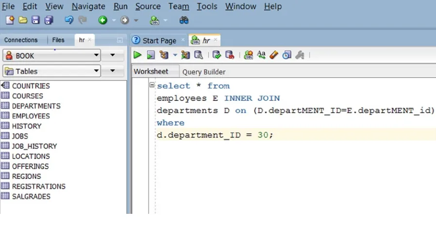
This chapter provides an introduction to the SQL language and one of two tools for working with it. Section 2.1 presents a high-level overview of the SQL language, which will give you an idea of the capabilities of this language. Then some important basic concepts of the SQL language are introduced in Section 2.2, such as constants, literals, variables, expressions, conditions, functions, operators, operands, and so on. Finally, in Section 2.3, this chapter provides a tour of SQL Developer, the main tool we recommend using to learn the SQL language. In order to maximize the benefits of any tool, you first must learn how to use it and to identify the main features available. In Chapter 11 the old, but still widely used SQL*Plus tool is explained in great detail. Even though many of the examples in this book are shown using SQL*Plus, feel free to use whichever tool you find most convenient.
This is the first chapter with real SQL statement examples. It thus would be beneficial for you to have access to an Oracle database and a schema with the seven case tables introduced in Chapter 1 and described in detail in Appendix A. You can find the scripts to create that schema in the download hosted from this book’s catalog page or the Source Code page on the Apress website.
We assume that Oracle is running; database (instance) startup and shutdown are normally tasks of a system or database administrator. Specific startup and shutdown procedures might be in place in your environment. However, if you are working with a stand-alone Oracle environment, and you have enough privileges, you can try the SQL*Plus
STARTUP command or use the GUI offered by Oracle Enterprise Manager to start up the database.
2.1 Overview of SQL
SQL (the abbreviation stands for Structured Query Language) is a language you can use in (at least) two different ways: interactively or embedded. Using SQL interactively means that you enter SQL commands via a keyboard, and you get the command results displayed on a terminal or computer screen. Using embedded SQL involves incorporating SQL commands within a program in a different programming language (such as Java or C). This book deals solely with interactive SQL usage.
Although SQL is called a query language, its possibilities go far beyond simply data retrieval. Normally, the SQL language is divided into the following four command categories:
Data definition (Data Definition Language, or DDL) •
Data manipulation (Data Manipulation Language, or DML) •
Retrieval •
Data Definition
The SQL data definition commands allow you to create, modify, and remove components of a database structure. Typical database structure components are tables, views, indexes, constraints, synonyms, sequences, and so on. Chapter 1 introduced tables, columns, and constraints; other database object types (such as views, indexes, synonyms, and sequences) will be introduced in later chapters.
Almost all SQL data definition commands start with one of the following three keywords: • CREATE, to create a new database object
• ALTER, to change an aspect of the structure of an existing database object • DROP, to drop (remove) a database object
For example, with the CREATE VIEW command, you can create views. With the ALTER TABLE command, you can change the structure of a table (for example by adding, renaming, or dropping a column). With the DROP INDEX
command, you can drop an index.
One of the strengths of an RDBMS is the fact that you can change the structure of a table without needing to change anything in your existing database application programs. For example, you can easily add a column or change its width with the ALTER TABLE command. In modern DBMSs such as Oracle, you can even do this while other database users or applications are connected and working on the database—like changing the wheels of a train at full speed. This property of an RDBMS is known as logical data independence (see Ted Codd’s rules, discussed in Chapter 1).
Data definition is covered in more detail in Chapters 3 and 7.
Data Manipulation and Transactions
Just as SQL data definition commands allow you to change the structure of a database, SQL data manipulation commands allow you to change the contents of your database. For this purpose, SQL offers three basic data manipulation commands:
• INSERT, to add rows to a table
• UPDATE, to change column values of existing rows • DELETE, to remove rows from a table
You can add rows to a table with the INSERT command in two ways. One way is to add rows one by one by specifying a list of column values in the VALUES clause of the INSERT statement. The other is to add one or more rows to a table based on a selection (and manipulation) of existing data in the database (called a subquery).