Herbert S. Wilf University of Pennsylvania Philadelphia, PA 19104-6395
Copyright Notice
Copyright 1994 by Herbert S. Wilf. This material may be reproduced for any educational purpose, multiple copies may be made for classes, etc. Charges, if any, for reproduced copies must be just enough to recover reasonable costs of reproduction. Reproduction for commercial purposes is prohibited. This cover page must be included in all distributed copies.
Internet Edition, Summer, 1994
This edition of Algorithms and Complexity is available at the web site<http://www/cis.upenn.edu/ wilf>. It may be taken at no charge by all interested persons. Comments and corrections are welcome, and should be sent [email protected]
Chapter 0: What This Book Is About
0.1 Background . . . 1
0.2 Hard vs. easy problems . . . 2
0.3 A preview . . . 4
Chapter 1: Mathematical Preliminaries 1.1 Orders of magnitude . . . 5
1.2 Positional number systems . . . 11
1.3 Manipulations with series . . . 14
1.4 Recurrence relations . . . 16
1.5 Counting . . . 21
1.6 Graphs . . . 24
Chapter 2: Recursive Algorithms 2.1 Introduction . . . 30
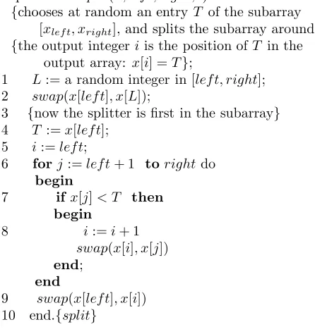
2.2 Quicksort . . . 31
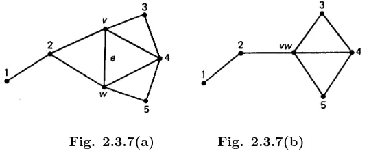
2.3 Recursive graph algorithms . . . 38
2.4 Fast matrix multiplication . . . 47
2.5 The discrete Fourier transform . . . 50
2.6 Applications of the FFT . . . 56
2.7 A review . . . 60
Chapter 3: The Network Flow Problem 3.1 Introduction . . . 63
3.2 Algorithms for the network flow problem . . . 64
3.3 The algorithm of Ford and Fulkerson . . . 65
3.4 The max-flow min-cut theorem . . . 69
3.5 The complexity of the Ford-Fulkerson algorithm . . . 70
3.6 Layered networks . . . 72
3.7 The MPM Algorithm . . . 76
3.8 Applications of network flow . . . 77
Chapter 4: Algorithms in the Theory of Numbers 4.1 Preliminaries . . . 81
4.2 The greatest common divisor . . . 82
4.3 The extended Euclidean algorithm . . . 85
4.4 Primality testing . . . 87
4.5 Interlude: the ring of integers modulon . . . 89
4.6 Pseudoprimality tests . . . 92
4.7 Proof of goodness of the strong pseudoprimality test . . . 94
4.8 Factoring and cryptography . . . 97
4.9 Factoring large integers . . . 99
5.1 Introduction . . . 104
5.2 Turing machines . . . 109
5.3 Cook’s theorem . . . 112
5.4 Some other NP-complete problems . . . 116
5.5 Half a loaf ... . . 119
5.6 Backtracking (I): independent sets . . . 122
5.7 Backtracking (II): graph coloring . . . 124
For the past several years mathematics majors in the computing track at the University of Pennsylvania have taken a course in continuous algorithms (numerical analysis) in the junior year, and in discrete algo-rithms in the senior year. This book has grown out of the senior course as I have been teaching it recently. It has also been tried out on a large class of computer science and mathematics majors, including seniors and graduate students, with good results.
Selection by the instructor of topics of interest will be very important, because normally I’ve found that I can’t cover anywhere near all of this material in a semester. A reasonable choice for a first try might be to begin with Chapter 2 (recursive algorithms) which contains lots of motivation. Then, as new ideas are needed in Chapter 2, one might delve into the appropriate sections of Chapter 1 to get the concepts and techniques well in hand. After Chapter 2, Chapter 4, on number theory, discusses material that is extremely attractive, and surprisingly pure and applicable at the same time. Chapter 5 would be next, since the foundations would then all be in place. Finally, material from Chapter 3, which is rather independent of the rest of the book, but is strongly connected to combinatorial algorithms in general, might be studied as time permits.
Throughout the book there are opportunities to ask students to write programs and get them running. These are not mentioned explicitly, with a few exceptions, but will be obvious when encountered. Students should all have the experience of writing, debugging, and using a program that is nontrivially recursive, for example. The concept of recursion is subtle and powerful, and is helped a lot by hands-on practice. Any of the algorithms of Chapter 2 would be suitable for this purpose. The recursive graph algorithms are particularly recommended since they are usually quite foreign to students’ previous experience and therefore have great learning value.
In addition to the exercises that appear in this book, then, student assignments might consist of writing occasional programs, as well as delivering reports in class on assigned readings. The latter might be found among the references cited in the bibliographies in each chapter.
I am indebted first of all to the students on whom I worked out these ideas, and second to a num-ber of colleagues for their helpful advice and friendly criticism. Among the latter I will mention Richard Brualdi, Daniel Kleitman, Albert Nijenhuis, Robert Tarjan and Alan Tucker. For the no-doubt-numerous shortcomings that remain, I accept full responsibility.
This book was typeset in TEX. To the extent that it’s a delight to look at, thank TEX. For the deficiencies in its appearance, thank my limitations as a typesetter. It was, however, a pleasure for me to have had the chance to typeset my own book. My thanks to the Computer Science department of the University of Pennsylvania, and particularly to Aravind Joshi, for generously allowing me the use of TEX facilities.
0.1 Background
An algorithm is a method for solving a class of problems on a computer. The complexity of an algorithm is the cost, measured in running time, or storage, or whatever units are relevant, of using the algorithm to solve one of those problems.
This book is about algorithms and complexity, and so it is about methods for solving problems on computers and the costs (usually the running time) of using those methods.
Computing takes time. Some problems take a very long time, others can be done quickly. Some problems seem to take a long time, and then someone discovers a faster way to do them (a ‘faster algorithm’). The study of the amount of computational effort that is needed in order to perform certain kinds of computations is the study of computationalcomplexity.
Naturally, we would expect that a computing problem for which millions of bits of input data are required would probably take longer than another problem that needs only a few items of input. So the time complexity of a calculation is measured by expressing the running time of the calculationas a function of some measure of the amount of data that is needed to describe the problem to the computer.
For instance, think about this statement: ‘I just bought a matrix inversion program, and it can invert an n×n matrix in just 1.2n3 minutes.’ We see here a typical description of the complexity of a certain
algorithm. The running time of the program is being given as a function of the size of the input matrix. A faster program for the same job might run in 0.8n3 minutes for an n
×nmatrix. If someone were to make a really important discovery (see section 2.4), then maybe we could actually lower the exponent, instead of merely shaving the multiplicative constant. Thus, a program that would invert ann×nmatrix in only 7n2.8minutes would represent a striking improvement of the state of the art.
For the purposes of this book, a computation that is guaranteed to take at mostcn3 time for input of
sizenwill be thought of as an ‘easy’ computation. One that needs at mostn10time is also easy. If a certain
calculation on ann×nmatrix were to require 2nminutes, then that would be a ‘hard’ problem. Naturally
some of the computations that we are calling ‘easy’ may take a very long time to run, but still, from our present point of view the important distinction to maintain will be the polynomial time guarantee or lack of it.
The general rule is that if the running time is at most a polynomial function of the amount of input data, then the calculation is an easy one, otherwise it’s hard.
Many problems in computer science are known to be easy. To convince someone that a problem is easy, it is enough to describe a fast method for solving that problem. To convince someone that a problem is hard is hard, because you will have to prove to them that it is impossible to find a fast way of doing the calculation. It will notbe enough to point to a particular algorithm and to lament its slowness. After all, thatalgorithm may be slow, but maybe there’s a faster way.
Matrix inversion is easy. The familiar Gaussian elimination method can invert ann×nmatrix in time at mostcn3.
To give an example of a hard computational problem we have to go far afield. One interesting one is called the ‘tiling problem.’ Suppose* we are given infinitely many identical floor tiles, each shaped like a regular hexagon. Then we can tile the whole plane with them,i.e., we can cover the plane with no empty spaces left over. This can also be done if the tiles are identical rectangles, but not if they are regular pentagons.
In Fig. 0.1 we show a tiling of the plane by identical rectangles, and in Fig. 0.2 is a tiling by regular hexagons.
That raises a number of theoretical and computational questions. One computational question is this. Suppose we are given a certain polygon, not necessarily regular and not necessarily convex, and suppose we have infinitely many identical tiles in that shape. Can we or can we not succeed in tiling the whole plane?
That elegant question has beenproved* to be computationally unsolvable. In other words, not only do we not know of any fast way to solve that problem on a computer, it has beenproved that there isn’t any
* See, for instance, Martin Gardner’s article inScientific American, January 1977, pp. 110-121.
Fig. 0.1: Tiling with rectangles
Fig. 0.2: Tiling with hexagons
way to do it, so even looking for an algorithm would be fruitless. That doesn’t mean that the question is hard for every polygon. Hard problems can have easy instances. What has been proved is that no single method exists that can guarantee that it will decide this question for every polygon.
The fact that a computationalproblemis hard doesn’t mean that every instance of it has to be hard. The problemis hard because we cannot devise an algorithm for which we can give aguaranteeof fast performance forallinstances.
Notice that the amount of input data to the computer in this example is quite small. All we need to input is the shape of the basic polygon. Yet not only is it impossible to devise a fast algorithm for this problem, it has been proved impossible to devise any algorithm at all that is guaranteed to terminate with a Yes/No answer after finitely many steps. That’sreallyhard!
0.2 Hard vs. easy problems
Let’s take a moment more to say in another way exactly what we mean by an ‘easy’ computation vs. a ‘hard’ one.
Think of an algorithm as being a little box that can solve a certain class of computational problems. Into the box goes a description of a particular problem in that class, and then, after a certain amount of time, or of computational effort, the answer appears.
A ‘fast’ algorithm is one that carries a guarantee of fast performance. Here are some examples. Example 1. It is guaranteed that if the input problem is described with B bits of data, then an answer will be output after at most6B3 minutes.
Example 2. It is guaranteed that every problem that can be input withB bits of data will be solved in at most0.7B15seconds.
A performance guarantee, like the two above, is sometimes called a ‘worst-case complexity estimate,’ and it’s easy to see why. If we have an algorithm that will, for example, sort any given sequence of numbers into ascending order of size (see section 2.2) it may find that some sequences are easier to sort than others. For instance, the sequence 1, 2, 7, 11, 10, 15, 20 is nearly in order already, so our algorithm might, if it takes advantage of the near-order, sort it very rapidly. Other sequences might be a lot harder for it to handle, and might therefore take more time.
So in some problems whose input bit string hasB bits the algorithm might operate in time 6B, and on others it might need, say, 10BlogB time units, and for still other problem instances of length B bits the algorithm might need 5B2 time units to get the job done.
Well then, what would the warranty card say? It would have to pick out the worst possibility, otherwise the guarantee wouldn’t be valid. It would assure a user that if the input problem instance can be described by B bits, then an answer will appear after at most 5B2 time units. Hence a performance guarantee is
equivalent to an estimation of the worst possible scenario: the longest possible calculation that might ensue ifB bits are input to the program.
Worst-case bounds are the most common kind, but there are other kinds of bounds for running time. We might give an average case bound instead (see section 5.7). That wouldn’t guarantee performance no worse than so-and-so; it would state that if the performance is averaged over all possible input bit strings of B bits, then the average amount of computing time will be so-and-so (as a function ofB).
Now let’s talk about the difference between easy and hard computational problems and between fast and slow algorithms.
A warranty that wouldnotguarantee ‘fast’ performance would contain some function of B that grows faster than any polynomial. Like eB, for instance, or like 2√B, etc. It is the polynomial time vs. not
necessarily polynomial time guarantee that makes the difference between the easy and the hard classes of problems, or between the fast and the slow algorithms.
It is highly desirable to work with algorithms such that we can give a performance guarantee for their running time that is at most a polynomial function of the number of bits of input.
An algorithm is slowif, whatever polynomialP we think of, there exist arbitrarily large values of B, and input data strings ofB bits, that cause the algorithm to do more thanP(B) units of work.
A computational problem istractableif there is a fast algorithm that will do all instances of it. A computational problem isintractableif it can be proved that there is no fast algorithm for it. Example 3. Here is a familiar computational problem and a method, or algorithm, for solving it. Let’s see if the method has a polynomial time guarantee or not.
The problem is this. Letnbe a given integer. We want to find out ifnisprime. The method that we choose is the following. For each integerm= 2,3, . . .,⌊√n⌋ we ask ifmdivides (evenly into)n. If all of the answers are ‘No,’ then we declarento be a prime number, else it is composite.
We will now look at thecomputational complexityof this algorithm. That means that we are going to find out how much work is involved in doing the test. For a given integernthe work that we have to do can be measured in units of divisions of a whole number by another whole number. In those units, we obviously will do about√nunits of work.
It seems as though this is a tractable problem, because, after all,√nis of polynomial growth in n. For instance, we do less thann units of work, and that’s certainly a polynomial inn, isn’t it? So, according to our definition of fast and slow algorithms, the distinction was made on the basis of polynomial vs. faster-than-polynomial growth of the work done with the problem size, and therefore this problem must be easy. Right? Well no, not really.
Reference to the distinction between fast and slow methods will show that we have to measure the amount of work doneas a function of the number of bits of input to the problem. In this example,nis not the number of bits of input. For instance, if n= 59, we don’t need 59 bits to describe n, but only 6. In general, the number of binary digits in the bit string of an integernis close to log2n.
So in the problem of this example, testing the primality of a given integern, the length of the input bit stringB is about log2n. Seen in this light, the calculation suddenly seems very long. A string consisting of
a mere log2n0’s and 1’s has caused our mighty computer to do about√nunits of work.
If we express the amount of work done as a function ofB,we find that the complexity of this calculation is approximately 2B/2, and that grows much faster than any polynomial function ofB.
Therefore, the method that we have just discussed for testing the primality of a given integer is slow. See chapter 4 for further discussion of this problem. At the present time no one has found a fast way to test for primality, nor has anyone proved that there isn’t a fast way. Primality testing belongs to the (well-populated) class of seemingly, but not provably, intractable problems.
but also, no one has proved the impossibility of doing so. It should be added that the entire area is vigorously being researched because of the attractiveness and the importance of the many unanswered questions that remain.
Thus, even though we just don’t know many things that we’d like to know in this field , it isn’t for lack of trying!
0.3 A preview
Chapter 1 contains some of the mathematical background that will be needed for our study of algorithms. It is not intended that reading this book or using it as a text in a course must necessarily begin with Chapter 1. It’s probably a better idea to plunge into Chapter 2 directly, and then when particular skills or concepts are needed, to read the relevant portions of Chapter 1. Otherwise the definitions and ideas that are in that chapter may seem to be unmotivated, when in fact motivation in great quantity resides in the later chapters of the book.
Chapter 2 deals with recursive algorithms and the analyses of their complexities.
Chapter 3 is about a problem that seems as though it might be hard, but turns out to be easy, namely the network flow problem. Thanks to quite recent research, there are fast algorithms for network flow problems, and they have many important applications.
In Chapter 4 we study algorithms in one of the oldest branches of mathematics, the theory of num-bers. Remarkably, the connections between this ancient subject and the most modern research in computer methods are very strong.
In Chapter 5 we will see that there is a large family of problems, including a number of very important computational questions, that are bound together by a good deal of structural unity. We don’t know if they’re hard or easy. We do know that we haven’t found a fast way to do them yet, and most people suspect that they’re hard. We also know that if any one of these problems is hard, then they all are, and if any one of them is easy, then they all are.
Chapter 1: Mathematical Preliminaries
1.1 Orders of magnitude
In this section we’re going to discuss the rates of growth of different functions and to introduce the five symbols of asymptotics that are used to describe those rates of growth. In the context of algorithms, the reason for this discussion is that we need a good language for the purpose of comparing the speeds with which different algorithms do the same job, or the amounts of memory that they use, or whatever other measure of the complexity of the algorithm we happen to be using.
Suppose we have a method of inverting square nonsingular matrices. How might we measure its speed? Most commonly we would say something like ‘if the matrix isn×nthen the method will run in time 16.8n3.’
Then we would know that if a 100×100 matrix can be inverted, with this method, in 1 minute of computer time, then a 200×200 matrix would require 23= 8 times as long, or about 8 minutes. The constant ‘16.8’
wasn’t used at all in this example; only the fact that the labor grows as the third power of the matrix size was relevant.
Hence we need a language that will allow us to say that the computing time, as a function ofn, grows ‘on the order ofn3,’ or ‘at most as fast as n3,’ or ‘at least as fast as n5logn,’ etc.
The new symbols that are used in the language of comparing the rates of growth of functions are the following five: ‘o’ (read ‘is little oh of’), ‘O’ (read ‘is big oh of’), ‘Θ’ (read ‘is theta of’), ‘∼’ (read ‘is asymptotically equal to’ or, irreverently, as ‘twiddles’), and ‘Ω’ (read ‘is omega of’).
Now let’s explain what each of them means.
Let f(x) andg(x) be two functions of x. Each of the five symbols above is intended to compare the rapidity of growth of f and g. If we say that f(x) = o(g(x)), then informally we are saying that f grows more slowly thang does when xis very large. Formally, we state the
Definition. We say thatf(x) =o(g(x)) (x→ ∞)iflimx→∞f(x)/g(x)exists and is equal to 0. Here are some examples:
(a) x2=o(x5)
(b) sinx=o(x)
(c) 14.709√x=o(x/2 + 7 cosx) (d) 1/x=o(1) (?)
(e) 23 logx=o(x.02)
We can see already from these few examples that sometimes it might be easy to prove that a ‘o’ relationship is true and sometimes it might be rather difficult. Example (e), for instance, requires the use of L’Hospital’s rule.
If we have two computer programs, and if one of them inverts n×nmatrices in time 635n3and if the
other one does so in timeo(n2.8) then we know that for all sufficiently large values of n the performance
guarantee of the second program will be superior to that of the first program. Of course, the first program might run faster on small matrices, say up to size 10,000×10,000. If a certain program runs in time n2.03and if someone were to produce another program for the same problem that runs in o(n2logn) time,
then that second program would be an improvement, at least in the theoretical sense. The reason for the ‘theoretical’ qualification, once more, is that the second program would be known to be superior only ifn were sufficiently large.
The second symbol of the asymptotics vocabulary is the ‘O.’ When we say that f(x) =O(g(x)) we mean, informally, thatf certainly doesn’t grow at a faster rate thang. It might grow at the same rate or it might grow more slowly; both are possibilities that the ‘O’ permits. Formally, we have the next
Definition. We say thatf(x) =O(g(x)) (x→ ∞)if∃C, x0such that|f(x)|< Cg(x) (∀x > x0).
The qualifier ‘x→ ∞’ will usually be omitted, since it will be understood that we will most often be interested in large values of the variables that are involved.
For example, it is certainly true that sinx=O(x), but even more can be said, namely that sinx=O(1). Also x3+ 5x2+ 77 cosx=O(x5) and 1/(1 +x2) = O(1). Now we can see how the ‘o’ gives more precise
sharper because not only does it tell us that the function is bounded when x is large, we learn that the function actually approaches 0 asx→ ∞.
This is typical of the relationship between Oando. It often happens that a ‘O’ result is sufficient for an application. However, that may not be the case, and we may need the more precise ‘o’ estimate.
The third symbol of the language of asymptotics is the ‘Θ.’
Definition. We say thatf(x) = Θ(g(x))if there are constants c1 >0, c2>0, x0 such that for allx > x0
it is true thatc1g(x)< f(x)< c2g(x).
We might then say thatf and g are of the same rate of growth, only the multiplicative constants are uncertain. Some examples of the ‘Θ’ at work are
(x+ 1)2= Θ(3x2) (x2+ 5x+ 7)/(5x3+ 7x+ 2) = Θ(1/x)
q
3 +√2x= Θ(x14)
(1 + 3/x)x= Θ(1).
The ‘Θ’ is much more precise than either the ‘O’ or the ‘o.’ If we know thatf(x) = Θ(x2), then we know
that f(x)/x2 stays between two nonzero constants for all sufficiently large values of x. The rate of growth
off is established: it grows quadratically withx.
The most precise of the symbols of asymptotics is the ‘∼.’ It tells us that not only dof andg grow at the same rate, but that in factf/g approaches 1 asx→ ∞.
Definition. We say thatf(x)∼g(x)iflimx→∞f(x)/g(x) = 1. Here are some examples.
x2+x ∼x2
(3x+ 1)4∼81x4 sin 1/x∼1/x (2x3+ 5x+ 7)/(x2+ 4)∼2x
2x+ 7 logx+ cosx ∼2x
Observe the importance of getting the multiplicative constants exactly right when the ‘∼’ symbol is used. While it is true that 2x2= Θ(x2), it is not true that 2x2
∼x2. It is, by the way, also true that 2x2= Θ(17x2),
but to make such an assertion is to use bad style since no more information is conveyed with the ‘17’ than without it.
The last symbol in the asymptotic set that we will need is the ‘Ω.’ In a nutshell, ‘Ω’ is the negation of ‘o.’ That is to say,f(x) = Ω(g(x)) means that it isnottrue thatf(x) =o(g(x)). In the study of algorithms for computers, the ‘Ω’ is used when we want to express the thought that a certain calculation takesat least so-and-so long to do. For instance, we can multiply together twon×n matrices in time O(n3). Later on
in this book we will see how to multiply two matrices even faster, in time O(n2.81). People know of even
faster ways to do that job, but one thing that we can be sure of is this: nobody will ever be able to write a matrix multiplication program that will multiply pairsn×nmatrices with fewer than n2 computational
steps, because whatever program we write will have to look at the input data, and there are 2n2 entries in
the input matrices.
Thus, a computing time ofcn2 is certainly alower bound on the speed of any possible general matrix
multiplication program. We might say, therefore, that the problem of multiplying twon×nmatrices requires Ω(n2) time.
Definition. We say thatf(x) = Ω(g(x))if there is an ǫ >0and a sequence x1, x2, x3, . . . → ∞such that ∀j: |f(xj)|> ǫg(xj).
Now let’s introduce a hierarchy of functions according to their rates of growth whenxis large. Among commonly occurring functions ofxthat grow without bound asx→ ∞, perhaps the slowest growing ones are functions like log logxor maybe (log logx)1.03or things of that sort. It is certainly true that log logx
→ ∞
asx→ ∞, but it takes its time about it. Whenx= 1,000,000, for example, log logxhas the value 2.6. Just a bit faster growing than the ‘snails’ above is logxitself. After all, log (1,000,000) = 13.8. So if we had a computer algorithm that could donthings in time lognand someone found another method that could do the same job in timeO(log logn), then the second method, other things being equal, would indeed be an improvement, butnmight have to be extremely large before you would notice the improvement.
Next on the scale of rapidity of growth we might mention the powers of x. For instance, think about x.01. It grows faster than logx, although you wouldn’t believe it if you tried to substitute a few values ofx
and to compare the answers (see exercise 1 at the end of this section).
How would weprovethat x.01grows faster than logx? By using L’Hospital’s rule.
Example. Consider the limit ofx.01/logxforx→ ∞. Asx→ ∞the ratio assumes the indeterminate form ∞/∞, and it is therefore a candidate for L’Hospital’s rule, which tells us that if we want to find the limit then we can differentiate the numerator, differentiate the denominator, and try again to letx→ ∞. If we do this, then instead of the original ratio, we find the ratio
.01x−.99/(1/x) =.01x.01
which obviously grows without bound asx→ ∞. Therefore the original ratiox.01/logxalso grows without
bound. What we have proved, precisely, is that logx=o(x.01), and therefore in that sense we can say that
x.01 grows faster thanlogx.
To continue up the scale of rates of growth, we meetx.2,x,x15,x15log2x, etc., and then we encounter
functions that grow faster thaneveryfixed power ofx, just as logxgrows slower than every fixed power of x.
Consider elog2
x. Since this is the same asxlogx it will obviously grow faster thanx1000, in fact it will
be larger thanx1000 as soon as logx >1000,i.e., as soon asx > e1000 (don’t hold your breath!).
Hence elog2
x is an example of a function that grows faster than every fixed power of x. Another such
example ise√x (why?).
Definition. A function that grows faster than xa, for every constant a, but grows slower than cx for
every constant c >1is said to be of moderately exponential growth. More precisely,f(x) is of moderately exponential growth if for everya >0we havef(x) = Ω(xa)and for everyǫ >0we have f(x) =o((1 +ǫ)x).
Beyond the range of moderately exponential growth are the functions that grow exponentially fast. Typical of such functions are (1.03)x, 2x,x97x, and so forth. Formally, we have the
Definition. A functionf is of exponential growth if there exists c >1such thatf(x) = Ω(cx)and there
existsdsuch thatf(x) =O(dx).
If we clutter up a function of exponential growth with smaller functions then we will not change the fact that it is of exponential growth. Thuse√x+2x/(x49+ 37) remains of exponential growth, becausee2xis,
all by itself, and it resists the efforts of the smaller functions to change its mind.
Beyond the exponentially growing functions there are functions that grow as fast as you might please. Liken!, for instance, which grows faster thancn for every fixed constantc, and like 2n2
, which grows much faster thann!. The growth ranges that are of the most concern to computer scientists are ‘between’ the very slowly, logarithmically growing functions and the functions that are of exponential growth. The reason is simple: if a computer algorithm requires more than an exponential amount of time to do its job, then it will probably not be used, or at any rate it will be used only in highly unusual circumstances. In this book, the algorithms that we will deal with all fall in this range.
Think about this one:
f(n) =
n
X
j=0
j2
= 12+ 22+ 32+· · ·+n2.
(1.1.1)
Thus, f(n) is the sum of the squares of the firstn positive integers. How fast does f(n) grow when n is large?
Notice at once that among the n terms in the sum that defines f(n), the biggest one is the last one, namely n2. Since there are n terms in the sum and the biggest one is only n2, it is certainly true that
f(n) =O(n3), and even more, thatf(n)
≤n3 for alln ≥1.
Suppose we wanted more precise information about the growth off(n), such as a statement likef(n)∼?. How might we make such a better estimate?
The best way to begin is to visualize the sum in (1.1.1) as shown in Fig. 1.1.1.
Fig. 1.1.1: How to overestimate a sum
In that figure we see the graph of the curvey=x2, in thex-y plane. Further, there is a rectangle drawn
over every interval of unit length in the range fromx= 1 tox=n. The rectangles all lieunder the curve. Consequently, the total area of all of the rectangles is smaller than the area under the curve, which is to say that
n−1
X
j=1
j2≤
Z n
1
x2dx
= (n3−1)/3.
(1.1.2)
If we compare (1.1.2) and (1.1.1) we notice that we have proved thatf(n)≤((n+ 1)3
−1)/3.
Now we’re going to get a lowerbound on f(n) in the same way. This time we use the setup in Fig. 1.1.2, where we again show the curve y=x2, but this time we have drawn the rectangles so they lieabove
the curve.
From the picture we see immediately that
12+ 22+· · ·+n2≥
Z n
0
x2dx =n3/3.
(1.1.3)
Now our functionf(n) has been bounded on both sides, rather tightly. What we know about it is that
∀n≥1 : n3/3≤f(n)≤((n+ 1)3−1)/3.
From this we have immediately thatf(n)∼n3/3, which gives us quite a good idea of the rate of growth of
Fig. 1.1.2: How to underestimate a sum
Let’s formulate a general principle, for estimating the size of a sum, that will make estimates like the above for us without requiring us each time to visualize pictures like Figs. 1.1.1 and 1.1.2. The general idea is that when one is faced with estimating the rates of growth of sums, then one should try to compare the sums with integrals because they’re usually easier to deal with.
Let a functiong(n) be defined for nonnegative integer values ofn, and suppose thatg(n) is nondecreasing. We want to estimate the growth of the sum
G(n) =
n
X
j=1
g(j) (n= 1,2, . . .). (1.1.4)
Consider a diagram that looks exactly like Fig. 1.1.1 except that the curve that is shown there is now the curvey =g(x). The sum of the areas of the rectangles is exactlyG(n−1), while the area under the curve between 1 andnis Rn
1 g(t)dt. Since the rectangles lie wholly under the curve, their combined areas cannot
exceed the area under the curve, and we have the inequality
G(n−1)≤
Z n
1
g(t)dt (n≥1). (1.1.5)
On the other hand, if we consider Fig. 1.1.2, where the graph is once more the graph of y = g(x), the fact that the combined areas of the rectangles is now not less thanthe area under the curve yields the inequality
G(n)≥
Z n
0
g(t)dt (n≥1). (1.1.6)
If we combine (1.1.5) and (1.1.6) we find that we have completed the proof of Theorem 1.1.1. Letg(x)be nondecreasing for nonnegativex. Then
Z n
0
g(t)dt≤
n
X
j=1
g(j)≤
Z n+1
1
g(t)dt. (1.1.7)
The above theorem is capable of producing quite satisfactory estimates with rather little labor, as the following example shows.
Letg(n) = lognand substitute in (1.1.7). After doing the integrals, we obtain
nlogn−n≤
n
X
j=1
We recognize the middle member above as logn!, and therefore by exponentiation of (1.1.8) we have
This is rather a good estimate of the growth ofn!, since the right member is only aboutnetimes as large as the left member (why?), when nis large.
By the use of slightly more precise machinery one can prove a better estimate of the size ofn! that is calledStirling’s formula, which is the statement that
x!∼(x e)
x√2xπ. (1.1.10)
Exercises for section 1.1
1. Calculate the values of x.01 and of logx forx= 10, 1000, 1,000,000. Find a single value of x >10 for
whichx.01>logx, and prove that your answer is correct.
2. Some of the following statements are true and some are false. Which are which? (a) (x2+ 3x+ 1)3
3. Each of the three sums below defines a function of x. Beneath each sum there appears a list of five assertions about the rate of growth, as x→ ∞, of the function that the sum defines. In each case state which of the five choices, if any, are true (note: more than one choice may be true).
h1(x) =
is a functionhsuch thatf =o(h) andh=o(g). Give an explicit construction for the function hin terms off andg.
6. {This exercise is a warmup for exercise 7.}Below there appear several mathematical propositions. In each case, write a proposition that is the negation of the given one. Furthermore, in the negation, do not use the word ‘not’ or any negation symbols. In each case the question is, ‘If thisisn’ttrue, then whatistrue?’
(a) ∃x >0∋f(x)6= 0 (b) ∀x >0, f(x)>0
(c) ∀x >0, ∃ǫ >0∋f(x)< ǫ (d) ∃x6= 0∋ ∀y <0, f(y)< f(x)
(e) ∀x∃y∋ ∀z:g(x)< f(y)f(z) (f) ∀ǫ >0∃x∋ ∀y > x:f(y)< ǫ
Can you formulate a general method for negating such propositions? Given a proposition that contains ‘∀,’ ‘∃,’ ‘∋,’ what rule would you apply in order to negate the proposition and leave the result in positive form (containing no negation symbols or ‘not’s).
7. In this exercise we will work out the definition of the ‘Ω.’
(a) Write out the precise definition of the statement ‘limx→∞h(x) = 0’ (use ‘ǫ’s). (b) Write out the negation of your answer to part (a), as a positive assertion.
(c) Use your answer to part (b) to give a positive definition of the assertion ‘f(x) 6= o(g(x)),’ and thereby justify the definition of the ‘Ω’ symbol that was given in the text.
8. Arrange the following functions in increasing order of their rates of growth, for largen. That is, list them so that each one is ‘little oh’ of its successor:
2√n, elogn3, n3.01,2n2, n1.6,logn3+ 1,√n!, n3 logn, n3logn,(log logn)3, n.52n,(n+ 4)12
9. Find a functionf(x) such thatf(x) =O(x1+ǫ) is true for every ǫ >0, but for which it is not true that
f(x) =O(x).
10. Prove that the statement ‘f(n) = O((2 +ǫ)n) for every ǫ > 0’ is equivalent to the statement ‘f(n) =
o((2 +ǫ)n) for every ǫ >0.’
1.2 Positional number systems
This section will provide a brief review of the representation of numbers in different bases. The usual decimal system represents numbers by using the digits 0,1, . . .,9. For the purpose of representing whole numbers we can imagine that the powers of 10 are displayed before us like this:
. . . ,100000,10000,1000,100,10,1.
Then, to represent an integer we can specify how many copies of each power of 10 we would like to have. If we write 237, for example, then that means that we want 2 100’s and 3 10’s and 7 1’s.
In general, if we write out the string of digits that represents a number in the decimal system, as dmdm−1· · ·d1d0, then the number that is being represented by that string of digits is
n=
m
X
i=0
di10i.
Now let’s try thebinary system. Instead of using 10’s we’re going to use 2’s. So we imagine that the powers of 2 are displayed before us, as
To represent a number we will now specify how many copies of each power of 2 we would like to have. For instance, if we write 1101, then we want an 8, a 4 and a 1, so this must be the decimal number 13. We will write
(13)10= (1101)2
to mean that the number 13, in the base 10, is the same as the number 1101, in the base 2.
In the binary system (base 2) the only digits we will ever need are 0 and 1. What that means is that if we use only 0’s and 1’s then we can represent every numbernin exactly one way. The unique representation of every number, is, after all, what we must expect and demand of any proposed system.
Let’s elaborate on this last point. If we were allowed to use more digits than just 0’s and 1’s then we would be able to represent the number (13)10 as a binary number in a whole lot of ways. For instance, we
might make the mistake of allowing digits 0, 1, 2, 3. Then 13 would be representable by 3·22+ 1·20 or by
2·22+ 2·21+ 1·20 etc.
So if we were to allow toomanydifferent digits, then numbers would be representable in more than one way by a string of digits.
If we were to allowtoo fewdifferent digits then we would find that some numbers have no representation at all. For instance, if we were to use the decimal system with only the digits 0,1, . . .,8, then infinitely many numbers would not be able to be represented, so we had better keep the 9’s.
The general proposition is this.
Theorem 1.2.1. Letb >1be a positive integer (the ‘base’). Then every positive integerncan be written in one and only one way in the form
n=d0+d1b+d2b2+d3b3+· · ·
if the digitsd0, d1, . . .lie in the range0≤di≤b−1, for alli.
Remark: The theorem says, for instance, that in the base 10 we need the digits 0,1,2, . . . ,9, in the base 2 we need only 0 and 1, in the base 16 we need sixteen digits, etc.
Proof of the theorem:Ifbis fixed, the proof is by induction onn, the number being represented. Clearly the number 1 can be represented in one and only one way with the available digits (why?). Suppose, inductively, that every integer 1,2, . . ., n−1 is uniquely representable. Now consider the integern. Define d=nmodb. Thendis one of thebpermissible digits. By induction, the numbern′= (n−d)/bis uniquely representable, say
n−d
b =d0+d1b+d2b
2+. . .
Then clearly,
n=d+n−d b b
=d+d0b+d1b2+d2b3+. . .
is a representation ofnthat uses only the allowed digits.
Finally, suppose thatnhas some other representation in this form also. Then we would have n=a0+a1b+a2b2+. . .
=c0+c1b+c2b2+. . .
Sincea0andc0are both equal tonmodb, they are equal to each other. Hence the numbern′= (n−a0)/b
has two different representations, which contradicts the inductive assumption, since we have assumed the truth of the result for alln′< n.
The bases b that are the most widely used are, aside from 10, 2 (‘binary system’), 8 (‘octal system’) and 16 (‘hexadecimal system’).
The octal system is popular because it provides a good way to remember and deal with the long bit strings that the binary system creates. According to the theorem, in the octal system the digits that we need are 0,1, . . .,7. For instance,
(735)8= (477)10.
The captivating feature of the octal system is the ease with which we can convert between octal and binary. If we are given the bit string of an integern, then to convert it to octal, all we have to do is to group the bits together in groups of three, starting with the least significant bit, then convert each group of three bits, independently of the others, into a single octal digit. Conversely, if the octal form of nis given, then the binary form is obtainable by converting each octal digit independently into the three bits that represent it in the binary system.
For example, given (1101100101)2. To convert this binary number to octal, we group the bits in threes,
(1)(101)(100)(101)
starting from the right, and then we convert each triple into a single octal digit, thereby getting
(1101100101)2= (1545)8.
If you’re a working programmer it’s very handy to use the shorter octal strings to remember, or to write down, the longer binary strings, because of the space saving, coupled with the ease of conversion back and forth.
The hexadecimal system (base 16) is like octal, only more so. The conversion back and forth to binary now uses groups of four bits, rather than three. In hexadecimal we will need, according to the theorem above, 16 digits. We have handy names for the first 10 of these, but what shall we call the ‘digits 10 through 15’ ? The names that are conventionally used for them are ‘A,’ ‘B,’...,‘F.’ We have, for example,
(A52C)16= 10(4096) + 5(256) + 2(16) + 12
= (42284)10
= (1010)2(0101)2(0010)2(1100)2
= (1010010100101100)2
= (1)(010)(010)(100)(101)(100) = (122454)8.
Exercises for section 1.2
1. Prove that conversion from octal to binary is correctly done by converting each octal digit to a binary triple and concatenating the resulting triples. Generalize this theorem to other pairs of bases.
2. Carry out the conversions indicated below. (a) (737)10= (?)3
(b) (101100)2= (?)16
(c) (3377)8= (?)16
(d) (ABCD)16= (?)10
(e) (BEEF)16= (?)8
1.3 Manipulations with series
In this section we will look at operations with power series, including multiplying them and finding their sums in simple form. We begin with a little catalogue of some power series that are good to know. First we have the finite geometric series
(1−xn)/(1−x) = 1 +x+x2+· · ·+xn−1. (1.3.1) This equation is valid certainly for all x 6= 1, and it remains true when x = 1 also if we take the limit indicated on the left side.
Why is (1.3.1) true? Just multiply both sides by 1−xto clear of fractions. The result is 1−xn= (1 +x+x2+x3+· · ·+xn−1)(1−x)
= (1 +x+x2+· · ·+xn−1)−(x+x2+x3+· · ·+xn) = 1−xn
and the proof is finished.
Now try this one. What is the value of the sum
9
X
j=0
3j?
Observe that we are looking at the right side of (1.3.1) withx= 3. Therefore the answer is (310
−1)/2. Try to get used to the idea that a series in powers ofx becomes a number ifxis replaced by a number, and if we know a formula for the sum of the series then we know the number that it becomes.
Here are some more series to keep in your zoo. A parenthetical remark like ‘(|x|<1)’ shows the set of values ofxfor which the series converges.
∞
X
k=0
xk = 1/(1−x) (|x|<1) (1.3.2)
ex= ∞
X
m=0
xm/m! (1.3.3)
sinx= ∞
X
r=0
(−1)rx2r+1/(2r+ 1)! (1.3.4)
cosx= ∞
X
s=0
(−1)sx2s/(2s)! (1.3.5)
log (1/(1−x)) = ∞
X
j=1
xj/j (|x|<1) (1.3.6)
Can you find a simple form for the sum (the logarithms are ‘natural’)
1 + log 2 + (log 2)2/2! + (log 2)3/3! + · · ·?
Hint: Look at (1.3.3), and replace xby log 2.
Aside from merely substituting values ofxinto known series, there are many other ways of using known series to express sums in simple form. Let’s think about the sum
We are reminded of the finite geometric series (1.3.1), but (1.3.7) is a little different because of the multipliers 1,2,3,4, . . ., N.
The trick is this. When confronted with a series that is similar to, but not identical with, a known series, write down the known series as an equation, with the series on one side and its sum on the other. Even though the unknown series involves a particular value ofx, in this case x= 2, keep the known series with its variable unrestricted. Then reach for an appropriate tool that will be applied to both sides of that equation, and whose result will be that the known series will have been changed into the one whose sum we needed.
In this case, since (1.3.7) reminds us of (1.3.1), we’ll begin by writing down (1.3.1) again,
(1−xn)/(1−x) = 1 +x+x2+· · ·+xn−1 (1.3.8) Don’t replacexby 2 yet, just walk up to the equation (1.3.8) carrying your tool kit and ask what kind of surgery you could do toboth sides of(1.3.8) that would be helpful in evaluating the unknown (1.3.7).
We are going to reach into our tool kit and pull out ‘d
dx.’ In other words, we are going todifferentiate
(1.3.8). The reason for choosing differentiation is that it will put the missing multipliers 1,2,3, . . ., N into (1.3.8). After differentiation, (1.3.8) becomes
If we rewrite the series using summation signs, it becomes
∞
X
j=2
1 j·3j.
Comparison with the series zoo shows great resemblance to the species (1.3.6). In fact, if we putx= 1/3 in (1.3.6) it tells us that
The desired sum (1.3.11) is the result of dropping the term withj = 1 from (1.3.12), which shows that the sum in (1.3.11) is equal to log (3/2)−1/3.
In general, suppose that f(x) =P
anxn is some series that we know. Then Pnanxn−1 =f′(x) and
P
nanxn=xf′(x). In other words, if thenthcoefficient is multiplied byn, then the function changes from
f to (xdxd)f. If we apply the rule again, we find that multiplying thenthcoefficient of a power series byn2
Similarly, multiplying the nth coefficient of a power series by np will change the sum from f(x) to
(xdxd )pf(x), but that’s not all. What happens if we multiply the coefficient ofxnby, say, 3n2+ 2n+ 5? If
the sum previously wasf(x), then it will be changed to{3(xd dx)
is therefore equal to{2(xd dx)
2+ 5
}{1/(1−x)}, and after doing the differentiations we find the answer in the form (7x2
−8x+ 5)/(1−x)3.
Here is the general rule: ifP(x) is any polynomial then
X
1. Find simple, explicit formulas for the sums of each of the following series. (a) P
3. Find the coefficient oftnin the series expansion of each of the following functions aboutt= 0. (a) (1 +t+t2)et
(b) (3t−t2) sint
(c) (t+ 1)2/(t−1)2
1.4 Recurrence relations
A recurrence relation is a formula that permits us to compute the members of a sequence one after another, starting with one or more given values.
Here is a small example. Suppose we are to find an infinite sequence of numbersx0, x1, . . .by means of
xn+1=cxn (n≥0; x0= 1). (1.4.1)
This relation tells us that x1=cx0, andx2=cx1, etc., and furthermore that x0= 1. It is then clear that
x1=c, x2=c2, . . . , xn=cn, . . .
We say that thesolutionof the recurrence relation (= ‘difference equation’) (1.4.1) is given byxn=cn
for all n≥ 0. Equation (1.4.1) is a first-orderrecurrence relation because a new value of the sequence is computed from just one preceding value (i.e.,xn+1 is obtained solely fromxn, and does not involvexn−1or
any earlier values).
Observe the format of the equation (1.4.1). The parenthetical remarks are essential. The first one ‘n≥0’ tells us for what values ofnthe recurrence formula is valid, and the second one ‘x0= 1’ gives the
starting value. If one of these is missing, the solution may not be uniquely determined. The recurrence relation
xn+1=xn+xn−1 (1.4.2)
The situation is rather similar to what happens in the theory of ordinary differential equations. There, if we omit initial or boundary values, then the solutions are determined only up to arbitrary constants.
Beyond the simple (1.4.1), the next level of difficulty occurs when we consider a first-order recurrence relation with a variable multiplier, such as
xn+1=bn+1xn (n≥0; x0 given). (1.4.3)
Now{b1, b2, . . .}is a given sequence, and we are being asked to find the unknown sequence {x1, x2, . . .}.
In an easy case like this we can write out the first fewx’s and then guess the answer. We find, successively, thatx1=b1x0, thenx2=b2x1=b2b1x0 andx3=b3x2=b3b2b1x0 etc. At this point we can guess that the
solution is
xn={ n
Y
i=1
bi}x0 (n= 0,1,2, . . .). (1.4.4)
Since that wasn’t hard enough, we’ll raise the ante a step further. Suppose we want to solve the first-order inhomogeneous(because xn= 0 for allnis not a solution) recurrence relation
xn+1=bn+1xn+cn+1 (n≥0; x0 given). (1.4.5)
Now we are being given two sequencesb1, b2, . . .andc1, c2, . . ., and we want to find thex’s. Suppose we
follow the strategy that has so far won the game, that is, writing down the first fewx’s and trying to guess the pattern. Then we would find thatx1=b1x0+c1, x2=b2b1x0+b2c1+c2, and we would probably tire
rapidly.
Here is a somewhat more orderly approach to (1.4.5). Though no approach will avoid the unpleasant form of the general answer, the one that we are about to describe at least gives a method that is much simpler than the guessing strategy, for many examples that arise in practice. In this book we are going to run into several equations of the type of (1.4.5), so a unified method will be a definite asset.
The first step is to define a new unknown function as follows. Let
xn=b1b2· · ·bnyn (n≥1; x0=y0) (1.4.6)
define a new unknown sequence y1, y2, . . .Now substitute forxnin (1.4.5), getting
b1b2· · ·bn+1yn+1=bn+1b1b2· · ·bnyn+cn+1.
We notice that the coefficients ofyn+1and ofynare the same, and so we divide both sides by that coefficient.
The result is the equation
yn+1=yn+dn+1 (n≥0; y0 given) (1.4.7)
where we have writtendn+1=cn+1/(b1· · ·bn+1). Notice that thed’s areknown.
We haven’t yet solved the recurrence relation. We have only changed to a new unknown function that satisfies a simpler recurrence (1.4.7). Now the solution of (1.4.7) is quite simple, because it says that eachy is obtained from its predecessor by adding the next one of thed’s. It follows that
yn=y0+ n
X
j=1
dj (n≥0).
We can now use (1.4.6) to reverse the change of variables to get back to the original unknownsx0, x1, . . .,
and find that
xn= (b1b2· · ·bn){x0+ n
X
j=1
dj} (n≥1). (1.4.8)
It is not recommended that the reader memorize the solution that we have just obtained. Itis recom-mended that the method by which the solution was found be mastered. It involves
(b) solve that one by summation and (c) go back to the original unknowns.
As an example, consider the first-order equation
xn+1= 3xn+n (n≥0; x0= 0). (1.4.9)
The winning change of variable, from (1.4.6), is to letxn= 3nyn. After substituting in (1.4.9) and simplifying,
we find
This is quite an explicit answer, but the summation can, in fact, be completely removed by the same method that you used to solve exercise 1(c) of section 1.3 (try it!).
That pretty well takes care of first-order recurrence relations of the form xn+1 =bn+1xn+cn+1, and
it’s time to move on to linear second order (homogeneous) recurrence relations with constant coefficients. These are of the form
xn+1=axn+bxn−1 (n≥1; x0and x1 given). (1.4.11)
If we think back to differential equations of second-order with constant coefficients, we recall that there are always solutions of the formy(t) = eαt where α is constant. Hence the road to the solution of such a
differential equation begins by trying a solution of that form and seeing what the constant or constantsα turn out to be.
Analogously, equation (1.4.11) calls for a trial solution of the formxn=αn. If we substitute xn=αn
in (1.4.11) and cancel a common factor ofαn−1we obtain a quadratic equation forα, namely
α2=aα+b. (1.4.12)
‘Usually’ this quadratic equation will have two distinct roots, sayα+ andα−, and then the general solution of (1.4.11) will look like
xn=c1αn++c2αn− (n= 0,1,2, . . .). (1.4.13)
The constants c1 andc2 will be determined so thatx0, x1 have their assigned values.
Example. The recurrence for the Fibonacci numbers is
Fn+1=Fn+Fn−1 (n≥1; F0=F1= 1). (1.4.14)
Following the recipe that was described above, we look for a solution in the formFn=αn. After substituting
in (1.4.14) and cancelling common factors we find that the quadratic equation forαis, in this case,α2=α+1.
If we denote the two roots byα+= (1 +√5)/2 andα− = (1−√5)/2, then the general solution to the Fibonacci recurrence has been obtained, and it has the form (1.4.13). It remains to determine the constants c1, c2 from the initial conditionsF0=F1= 1.
The Fibonacci numbers are in fact 1,1,2,3,5,8,13,21,34, . . . It isn’t even obvious that the formula (1.4.15) gives integer values for theFn’s. The reader should check that the formula indeed gives the first few
Fn’s correctly.
Just to exercise our newly acquired skills in asymptotics, let’s observe that since (1 +√5)/2>1 and
|(1−√5)/2|<1, it follows that whennis large we have
Fn∼((1 + √
5)/2)n+1/√5.
The process of looking for a solution in a certain form, namely in the formαn, is subject to the same
kind of special treatment, in the case of repeated roots, that we find in differential equations. Corresponding to adoublerootαof the associated quadratic equationα2=aα+bwe would find two independent solutions
αnandnαn, so the general solution would be in the formαn(c
1+c2n).
Example. Consider the recurrence
xn+1= 2xn−xn−1 (n≥1; x0= 1; x1= 5). (1.4.16)
If we try a solution of the type xn=αn, then we find that αsatisfies the quadratic equationα2 = 2α−1.
Hence the ‘two’ roots are 1 and 1. The general solution isxn= 1n(c1+nc2) =c1+c2n. After inserting the
given initial conditions, we find that
x0= 1 =c1; x1= 5 =c1+c2
If we solve for c1 and c2 we obtainc1 = 1, c2 = 4, and therefore the complete solution of the recurrence
(1.4.16) is given byxn= 4n+ 1.
Now let’s look at recurrent inequalities, like this one:
xn+1≤xn+xn−1+n2 (n≥1; x0= 0; x1= 0). (1.4.17)
The question is, what restriction is placed on the growth of the sequence{xn}by (1.4.17)?
By analogy with the case of difference equations with constant coefficients, the thing to try here is xn≤Kαn. So suppose it is true thatxn≤Kαnfor alln= 0,1,2, . . ., N. Then from (1.4.17) with n=N
we find
xN+1≤KαN +KαN−1+N2.
Letcbe the positive real root of the equationc2=c+ 1, and suppose thatα > c. Thenα2> α+ 1 and so
α2
−α−1 =t, say, wheret >0. Hence
xN+1≤KαN−1(1 +α) +N2
=KαN−1(α2−t) +N2 =KαN+1−(tKαN−1−N2).
(1.4.18)
In order to insure thatxN+1< KαN+1 what we need is for tKαN−1> N2. Hence as long as we choose
K >max
N≥2
N2/tαN−1 , (1.4.19)
in which the right member is clearly finite, the inductive step will go through.
The conclusion is that (1.4.17) implies that for every fixedǫ >0,xn=O((c+ǫ)n), wherec= (1+ √
Theorem 1.4.1. Let a sequence {xn}satisfy a recurrent inequality of the form
xn+1≤b0xn+b1xn−1+· · ·+bpxn−p+G(n) (n≥p)
wherebi≥0 (∀i),Pbi>1. Further, letc be the positive real root of * the equa tioncp+1=b0cp+· · ·+bp.
Finally, suppose G(n) =o(cn). Then for every fixed ǫ >0we have x
n=O((c+ǫ)n).
Proof: Fix ǫ > 0, and let α =c+ǫ, where c is the root of the equation shown in the statement of the theorem. Sinceα > c, if we let
t=αp+1−b0αp− · · · −bp
thent >0. Finally, define
K= max
|x0|,|x1|
α , . . . ,
|xp|
αp , maxn≥p
G(n)
tαn−p
.
ThenKis finite, and clearly|xj| ≤Kαj forj≤p. We claim that|xn| ≤Kαnfor alln, which will complete
the proof.
Indeed, if the claim is true for 0,1,2, . . ., n, then
|xn+1| ≤b0|x0|+· · ·+bp|xn−p|+G(n) ≤b0Kαn+· · ·+bpKαn−p+G(n)
=Kαn−p{b0αp+· · ·+bp}+G(n)
=Kαn−p {αp+1
−t}+G(n) =Kαn+1
− {tKαn−p
−G(n)}
≤Kαn+1
.
Exercises for section 1.4
1. Solve the following recurrence relations (i) xn+1=xn+ 3 (n≥0; x0= 1)
(ii) xn+1=xn/3 + 2 (n≥0; x0= 0)
(iii) xn+1= 2nxn+ 1 (n≥0; x0= 0)
(iv) xn+1= ((n+ 1)/n)xn+n+ 1 (n≥1; x1= 5)
(v) xn+1=xn+xn−1 (n≥1;x0= 0; x1= 3)
(vi) xn+1= 3xn−2xn−1 (n≥1;x0= 1; x1= 3)
(vii) xn+1= 4xn−4xn−1 (n≥1; x0= 1; x1=ξ)
2. Find x1 if the sequence x satisfies the Fibonacci recurrence relation and if furthermore x0 = 1 and
xn=o(1) (n→ ∞).
3. Let xn be the average number of trailing 0’s in the binary expansions of all integers 0,1,2, . . .,2n−1.
Find a recurrence relation satisfied by the sequence {xn}, solve it, and evaluate limn→∞xn.
4. For what values ofaandbis it true that no matter what the initial valuesx0,x1are, the solution of the
recurrence relationxn+1=axn+bxn−1 (n≥1) is guaranteed to be o(1) (n→ ∞)?
5. Supposex0= 1,x1= 1, and for alln≥2 it is true thatxn+1≤xn+xn−1. Is it true that ∀n:xn≤Fn?
Prove your answer.
6. Generalize the result of exercise 5, as follows. Suppose x0 = y0 and x1 = y1, where yn+1 = ayn+
byn−1 (∀n≥1). If furthermore, xn+1 ≤axn+bxn−1 (∀n≥1), can we conclude that ∀n:xn≤yn? If
not, describe conditions onaandbunder which that conclusion would follow.
7. Find the asymptotic behavior in the formxn∼? (n→ ∞) of the right side of (1.4.10).
8. Write out a complete proof of theorem 1.4.1.
9. Show by an example that the conclusion of theorem 1.4.1 may be false if the phrase ‘for every fixed ǫ >0. . .’ were replaced by ‘for every fixedǫ≥0. . ..’
10. In theorem 1.4.1 we find the phrase ‘... the positive real root of ...’ Prove that this phrase is justified, in that the equation shown always has exactly one positive real root. Exactly what special properties of that equation did you use in your proof?
1.5 Counting
For a given positive integer n, consider the set {1,2, . . .n}. We will denote this set by the symbol [n], and we want to discuss the number of subsets of various kinds that it has. Here is a list of all of the subsets of [2]: ∅,{1},{2},{1,2}. There are 4 of them.
We claim that the set [n] has exactly 2nsubsets.
To see why, notice that we can construct the subsets of [n] in the following way. Either choose, or don’t choose, the element ‘1,’ then either choose, or don’t choose, the element ‘2,’ etc., finally choosing, or not choosing, the element ‘n.’ Each of then choices that you encountered could have been made in either of 2 ways. The totality ofnchoices, therefore, might have been made in 2ndifferent ways, so that is the number
of subsets that a set ofnobjects has.
Next, suppose we haven distinct objects, and we want to arrange them in a sequence. In how many ways can we do that? For the first object in our sequence we may choose any one of the n objects. The second element of the sequence can be any of the remainingn−1 objects, so there are n(n−1) possible ways to make the first two decisions. Then there are n−2 choices for the third element, and so we have n(n−1)(n−2) ways to arrange the first three elements of the sequence. It is no doubt clear now that there are exactlyn(n−1)(n−2)· · ·3·2·1 =n! ways to form the whole sequence.
Of the 2n subsets of [n], how many have exactly k objects in them? The number of elements in a
set is called its cardinality. The cardinality of a set S is denoted by|S|, so, for example,|[6]|= 6. A set whose cardinality iskis called a ‘k-set,’ and a subset of cardinalitykis, naturally enough, a ‘k-subset.’ The question is, for how many subsets S of [n] is it true that|S|=k?
We can construct k-subsets S of [n] (written ‘S ⊆ [n]’) as follows. Choose an element a1 (n possible
choices). Of the remaining n−1 elements, choose one (n−1 possible choices), etc., until a sequence of k different elements have been chosen. Obviously there were n(n−1)(n−2)· · ·(n−k+ 1) ways in which we might have chosen that sequence, so the number of ways to choose an (ordered) sequence ofkelements from [n] is
n(n−1)(n−2)· · ·(n−k+ 1) =n!/(n−k)!.
But there are more sequences ofkelements than there arek-subsets, because any particulark-subsetS will correspond tok! different ordered sequences, namely all possible rearrangements of the elements of the subset. Hence the number ofk-subsets of [n] is equal to the number ofk-sequences divided byk!. In other words, there are exactlyn!/k!(n−k)!k-subsets of a set ofnobjects.
The quantitiesn!/k!(n−k)! are the famousbinomial coefficients, and they are denoted by
n
It is convenient to define nk
Theorem 1.5.1. For each n≥0, a set ofn objects has exactly2nsubsets, and of these, exactly n
Since every subset of [n] hassomecardinality, it follows that
n
In view of the convention that we adopted, we might have written (1.5.2) asP
k n k
= 2n, with no restriction
on the range of the summation index k. It would then have been understood that the range of k is from
−∞to∞, and that the binomial coefficient nk
vanishes unless 0≤k≤n. In Table 1.5.1 we show the values of some of the binomial coefficients nk
. The rows of the table are thought of as labelled ‘n = 0,’ ‘n = 1,’ etc., and the entries within each row refer, successively, to k= 0,1, . . ., n. The table is called ‘Pascal’s triangle.’
Here are some facts about the binomial coefficients:
(a) Each row of Pascal’s triangle is symmetric about the middle. That is,
n
(c) Each entry is equal to the sum of the two entries that are immediately above it in the triangle. The proof of (c) above can be interesting. What it says about the binomial coefficients is that
n
There are (at least) two ways to prove (1.5.3). The hammer-and-tongs approach would consist of expanding each of the three binomial coefficients that appears in (1.5.3), using the definition (1.5.1) in terms of factorials, and then cancelling common factors to complete the proof.
That would work (try it), but here’s another way. Contemplate (this proof is by contemplation) the totality ofk-subsets of [n]. The number of them is on the left side of (1.5.3). Sort them out into two piles: those k-subsets that contain ‘1’ and those that don’t. If a k-subset of [n] contains ‘1,’ then its remaining k−1 elements can be chosen in nk−−11
Thebinomial theorem is the statement that∀n≥0 we have
Proof: By induction onn. Eq. (1.5.4) is clearly true whenn= 0, and if it is true for some nthen multiply both sides of (1.5.4) by (1 +x) to obtain
Now let’s ask how big the binomial coefficients are, as an exercise in asymptotics. We will refer to the coefficients in rownof Pascal’s triangle, that is, to
n
as the coefficients oforder n. Then, by (1.5.2) (or by (1.5.4) withx= 1), the sum of all of the coefficients of order nis 2n. It is also fairly apparent, from an inspection of Table 1.5.1, that the largest one(s) of the
coefficients of order nis (are) the one(s) in the middle.
More precisely, ifnis odd, then the largest coefficients of order nare (n−n1)/2
and (n+1)/2n
, whereas ifnis even, the largest one is uniquely n/2n
.
It will be important, in some of the applications to algorithms later on in this book, for us to be able to pick out the largest term in a sequence of this kind, so let’s see how we could prove that the biggest coefficients are the ones cited above.
Fornfixed, we will compute the ratio of the (k+ 1)st coefficient of ordernto thekth. We will see then
that the ratio is larger than 1 ifk <(n−1)/2 and is<1 ifk >(n−1)/2. That, of course, will imply that the (k+ 1)st coefficient is bigger than the kth, for such k, and therefore that the biggest one(s) must be in
the middle.
OK, the biggest coefficients are in the middle, but how big are they? Let’s suppose thatnis even, just to keep things simple. Then the biggest binomial coefficient of order nis
where we have used Stirling’s formula (1.1.10).
Equation (1.5.5) shows that the single biggest binomial coefficient accounts for a very healthy fraction of the sum ofallof the coefficients of order n. Indeed, the sum of all of them is 2n, and the biggest one is ∼p
2/nπ2n. Whennis large, therefore, the largest coefficient contributes a fraction∼p
2/nπof the total. If we think in terms of the subsets that these coefficients count, what we will see is that a large fraction of all of the subsets of ann-set have cardinalityn/2, in fact Θ(n−.5) of them do. This kind of probabilistic
thinking can be very useful in the design and analysis of algorithms. If we are designing an algorithm that deals with subsets of [n], for instance, we should recognize that a large percentage of the customers for that algorithm will have cardinalities near n/2, and make every effort to see that the algorithm is fast for such subsets, even at the expense of possibly slowing it down on subsets whose cardinalities are very small or very large.
Exercises for section 1.5
1. How many subsets of even cardinality does [n] have?
2. By observing that (1 +x)a(1 +x)b = (1 +x)a+b, prove that the sum of the squares of all binomial
coefficients of order nis 2nn
.
3. Evaluate the following sums in simple form. (i) Pn
4. Find, by direct application of Taylor’s theorem, the power series expansion off(x) = 1/(1−x)m+1about
the origin. Express the coefficients as certain binomial coefficients. 5. Complete the following twiddles.
6. How many ordered pairs of unequal elements of [n] are there? 7. Which one of the numbers{2j n
A graph is a collection ofvertices, certain unordered pairs of which are called itsedges. To describe a particular graph we first say what its vertices are, and then we say which pairs of vertices are its edges. The set of vertices of a graphGis denoted byV(G), and its set of edges isE(G).
Ifv andw are vertices of a graphG, and if (v, w) is an edge ofG, then we say that vertices v,w are adjacentinG.
Consider the graphGwhose vertex set is{1,2,3,4,5}and whose edges are the set of pairs (1,2), (2,3), (3,4), (4,5), (1,5). This is a graph of 5 vertices and 5 edges. A nice way to present a graph to an audience is to draw a picture of it, instead of just listing the pairs of vertices that are its edges. To draw a picture of a graph we would first make a point for each vertex, and then we would draw an arc between two verticesv andwif and only if (v, w) is an edge of the graph that we are talking about. The graphGof 5 vertices and 5 edges that we listed above can be drawn as shown in Fig. 1.6.1(a). It could also be drawn as shown in Fig. 1.6.1(b). They’re both the same graph. Only the pictures are different, but the pictures aren’t ‘really’ the graph; the graph is the vertex list and the edge list. The pictures are helpful to us in visualizing and remembering the graph, but that’s all.