The Lattice Structure of Connection Preserving
Deformations for
q
-Painlev´
e Equations I
Christopher M. ORMEROD
La Trobe University, Department of Mathematics and Statistics, Bundoora VIC 3086, Australia
E-mail: [email protected]
Received November 26, 2010, in final form May 03, 2011; Published online May 07, 2011
doi:10.3842/SIGMA.2011.045
Abstract. We wish to explore a link between the Lax integrability of theq-Painlev´e equa-tions and the symmetries of theq-Painlev´e equations. We shall demonstrate that the con-nection preserving deformations that give rise to theq-Painlev´e equations may be thought of as elements of the groups of Schlesinger transformations of their associated linear prob-lems. These groups admit a very natural lattice structure. Each Schlesinger transformation induces a B¨acklund transformation of theq-Painlev´e equation. Each translational B¨acklund transformation may be lifted to the level of the associated linear problem, effectively showing that each translational B¨acklund transformation admits a Lax pair. We will demonstrate this framework for the q-Painlev´e equations up to and includingq-PVI.
Key words: q-Painlev´e; Lax pairs;q-Schlesinger transformations; connection; isomonodromy
2010 Mathematics Subject Classification: 34M55; 39A13
1
Introduction and outline
The discrete Painlev´e equations are second order non-linear non-autonomous difference equa-tions admitting the the Painlev´e equaequa-tions as continuum limits [22]. They are considered integrable by the integrability criterion of singularity confinement [22], solvability via asso-ciated linear problems [21] and have zero algebraic entropy [2]. There are three classes of discrete Painlev´e equations: the additive difference equations, q-difference equations and ellip-tic difference equations. This classification is in accordance with the way in which the non-autonomous variable evolves with each application of the iterative scheme. The aim of this article is to derive a range of symmetries of the consideredq-difference Painlev´e equations using the framework of their associated linear problems.
The discovery of the solvability of a q-Painlev´e equation via an associated linear problem was established by Papageorgiou et al. [21]. It was found that a q-Painlev´e equation can be equivalent to the compatibility condition between two systems of linear q-difference equations, given by
Y(qx, t) =A(x, t)Y(x, t), (1.1a)
Y(x, qt) =B(x, t)Y(x, t), (1.1b)
by (1.1b). This theory also led to the discovery of the q-analogue the sixth Painlev´e equation in an analogous manner to the classical result of Fuchs [9,8].
There was one unresolved issue in the explanation of the emergence of discrete Painlev´e type systems, and this was related to the emergence, and definition, of B(x, t). Unlike the theory of monodromy preserving deformations and the surfaces of initial conditions where there exists just one canonical Hamiltonian flow [27, 13], there are many ways to preserve the connection matrix. According to the existing framework, one may determine B(x, t) from a known change in the discrete analogue of monodromy data, i.e., the characteristic data. However, we would argue that this known change is not canonical, or unique. That is to say that by considering all possible changes in the characteristic data, one formulates a system of Schlesinger transforma-tions inducing a system of B¨acklund transformatransforma-tions of the Painlev´e equation. A particular case of this theory was studied by the author in connection with the q-difference equation satisfied by the Big q-Laguerre polynomials [20].
This concept is not entirely new, one only needs to examine Jimbo and Miwa’s second pa-per [11] to see a set of discrete transformations, known as Schlesinger transformations, specified for the Painlev´e equations. These Schlesinger transformations can be thought of as a discrete group of monodromy preserving evolutions, in which various elements of the monodromy data are shifted by integer amounts. The compatibility between the discrete evolution and the con-tinuous flow induces a B¨acklund transformation of the Painlev´e equation, which appear in the associated linear problem, and in some cases, induce the evolution of some discrete Painlev´e equations of additive type [15].
We will show the same type of transformations for systems ofq-difference equations describe similar transformations. We consider systems of transformations in which (1.1a) is quadratic. There are only a finite number of cases in which A(x) is quadratic, and these cases cover the
q-Painlev´e equations up to and including theq-analogue of the sixth Painlev´e equation [14]. We will consider the set of transformations of the associated linear problems for the exceptional
q-Painlev´e equations in a separate article as we have preliminary results, including a Lax pair for one of these equations that seems distinct from those that have appeared in [31] and [25].
These transformations may be derived in an analogous manner to the differential case. If one knows formal expansions of the solutions of (1.1a) atx= 0 andx=∞, then one may formulate the Schlesinger transformations directly in terms of the expansions. Formal expansions for regularq-difference equations are well established in the integrable community [4,14], however, many associated linear problems forq-Painlev´e equations fail to be regular at 0 or∞. Hence, it is another goal of this article to apply the more general expansions provided by Adams [1] and Guenther [5] to derive the required Schlesinger equations. These expansions seem to be not as well established, however, all known examples of connection preserving deformations seem to fit nicely a framework that encompasses the regular and irregular cases [14, 17, 21]. In previous studies, such as those by by Sakai [24,14], B(x, t) from (1.1b) and the Painlev´e equations seem to have been derived from an overdetermined set of compatibility conditions. In an analogous manner to the continuous case, the formal solutions obtained may or may not converge in any given region of the complex plane [28].
The most important distinction we wish to make here is the absence of a variable t. We remark that this should be seen as a consistent trend in the studies of discrete Painlev´e equations, whereby the framework of Sakai [23] and the work of Noumi et al. [18] show us that we should consider the B¨acklund transformations and discrete Painlev´e equations on the same footing.
2
q
-special functions
A general theory of specialq-difference equations, with particular interest in basic hypergeomet-ric series, may be found in the book by Gasper and Rahman [10]. The work of Sauloy and Ramis provide some insight as to how these q-special functions both relate to the special solutions of the linear problems and the connection matrix [26, 7], as does the work of van der Put and Singer [29, 30]. For the following theory, it is convenient to fix a q ∈ C such that |q| < 1, in order to have given functions define analytic functions around 0 or ∞.
We start by defining theq-Pochhammer symbol [10], given by
(a, q)k=
k
Q
n=1
1−aqn−1
fork∈N, ∞
Q
n=1
1−aqn−1
fork=∞,
1 fork= 0.
We note that (a, q)∞ satisfies
(qx;q)∞=
1
1−x(x;q)∞,
or equivalently,
x q;q
∞
=
1− x
q
(x;q)∞.
We define a fundamental building block; the Jacobi theta function [10], given by the bi-infinite expansion
θq(x) =
X
n∈Z
q(n2)xn,
which satisfies theq-difference equation
xθq(qx) =θq(x).
The second function we require to describe the asymptotics of the solutions of (1.1a) is the
q-character, given by
eq,c(x) =
θq(x)θq(c) θq(xc)
,
which satisfies
eq,c(qx) =ceq,c(x), eq,qc(x) =xeq,c(x).
Using the above functions, we are able to solve any one dimensional problem.
3
Connection preserving deformations
We will take a deeper look into systems of linearq-difference equations of the form
where theai(x) are rational functions. One may easily express a system of this form as a matrix
equation of the form
Y(qx) =A(x)Y(x),
whereA(x) is some rational matrix. We quote the theorem of Adams [1] suitably translated for matrix equations by Birkhoff [5] in the revised language of Sauloy et al. [26,29].
Theorem 3.1. Under general conditions, the system possesses formal solutions given by
Y0(x) = ˆY0(x)D0(x), Y∞(x) = ˆY∞(x)D∞(x), (3.1)
where Yˆ0(x) and Yˆ∞(x) are series expansions in x around x= 0 and x=∞ respectively and
D0(x) = diag
eq,λi(x)
θq(x)νi
, D∞(x) = diag
eq,κi(x)
θq(x)νi
.
Given the existence and convergence of these solutions, we may form the connection matrix, similar to that of difference equations [3], given by
P(x) =Y∞(x)Y0(x)−1.
In a similar manner to monodromy preserving deformations, we identify a discrete set of cha-racteristic data, namely
M =
κ1 . . . κn
λ1 . . . λn a1 . . . am
.
Defining this characteristic data may not uniquely define A(x) in general. In the problems we consider, which are also those problems considered previously in the work of Sakai [14], Murata [17] and Yamada [31], the characteristic data defines a three dimensional linear algebraic group as a system of two first order linear q-difference equations, but is two dimensional as one second orderq-difference equation. The gauge freedom disappears when one extracts the second order q-difference equation from the system of two first order q-difference equations. Let us suppose the linear algebraic group is of dimension d, then let us introduce variablesy1, y2,. . ., yd, which parameterize the linear algebraic group. We may now set a co-ordinate system for
this linear algebraic group, hence, we write
MA=
κ1 . . . κn
λ1 . . . λn a1 . . . am
:y1, . . . , yd
, (3.2)
as defining a matrix A.
By considering the determinant of the left hand side of (1.1a) and the fundamental solutions specified by (3.1), one is able to show
n
Y
i=1 κi
m
Y
j=1
(−aj) = n
Y
i=1
λi, (3.3)
which forms a constraint on the characteristic data.
We now explore connection preserving deformations [14]. LetR(x) be a rational matrix in x, then we apply a transformation Y →Y˜ by the matrix equation
˜
The matrix ˜Y satisfies a matrix equation of the form (1.1a), given by
˜
Y(qx) =
R(qx)A(x)R(x)−1˜
Y(x) = ˜A(x) ˜Y(x). (3.5)
We note that ifR(x) is rational and invertible, then
˜
P(x) = ( ˜Y∞(x))−1Y˜0(x) = (R(x)Y∞(x))−1R(x)Y0(x)
= (Y∞(x)) −1
R(x)−1R(x)Y0(x) =Y∞(x)Y0(x),
hence, the system defined by
˜
Y(qx) = ˜A(x) ˜Y(x),
is a system of linearq-difference equations that possesses the same connection matrix. However, the left action of R(x) may have the following effects: The transformation may
• change the asymptotic behavior of the fundamental solutions at x =∞ by letting κi → qnκ
i;
• change the asymptotic behavior of the fundamental solutions atx= 0 by lettingλi→qnλi;
• change the position of a root of the determinant by letting ai →qnai.
We use the same co-ordinate system for ˜A(x) as we did forA(x) via (3.2), giving
MA˜ =
˜
κ1 . . . ˜κn
˜
λ1 . . . λ˜n a˜1 . . . ˜am
: ˜y1, . . . ,y˜d
.
Naturally, R(x) is a function of the characteristic data and the yi, hence, we write
R(x) = ˜Y0(x)Y0(x)−1= ˜Y∞(x)Y∞(x)−1=R(x;yi,y˜i, κj,κ˜j,λ˜l, λl, an,˜an).
An alternate characterization of (3.5) is the compatibility condition resulting the consistency of (3.4) with (1.1a), which gives
˜
A(x)R(x) =R(qx)A(x), (3.6)
which has appeared many times in the literature [14,21,24]. Given a suitable parameterization, we obtain a rational map on the co-ordinate system for A(x):
T : MA→MA˜,
For eachi= 1, . . . , d, we use (3.6) to find a rational mappingφi such that
˜
yi =φi(MA),
where MA includes all of the variables in (3.2).
We now draw further correspondence with the framework of Jimbo and Miwa [11]. Let
{µ1, . . . , µK} be a collection of elements in the characteristic data, and {m1, . . . , mK} be a set
of integers, then we define the transformation
Tµm1
1 ,...,µmKK : MA→MA˜,
to be the transformation that multiplies µi by qmi leaving all other characteristic data fixed.
The mi have to be chosen so that MA˜ satisfies (3.3). The group of Schlesinger
transforma-tions, GA, is the set of these transformation with the operation of composition
GA=hTµm1
This group is generated by a set of elementary Schlesinger transformations which only alter two variables, i.e.,K = 2. For example, if wish to multiplyκ1byqanda1byq−1, so to preserve (3.3),
this would be the elementary transformation Tκ1,a−1
1 . Since the subscripts define the change in
characteristic data, we need only specify the relation between theyi and ˜yi, hence, we will write
Tµm1
1 ,...,µmKK : ˜y1 =φ1(MA), . . . , y˜d=φd(MA).
We will denote matrix that induces the transformation Tµm1
1 ,...,µmKK by Rµ m1
1 ,...,µmKK so that the transformation MA→MA˜ is specified by the transformation of the linear problem given by
˜
Y(x) =Rµm1
1 ,...,µmKK (x)Y(x).
The goal of the the later sections will be to construct a set of elementary Schlesinger transfor-mations that generate GA and describe the correspondingR matrices.
4
q
-Painlev´
e equations
We now look at the group of Schlesinger transformations for theq-Painlev´e equations. In accor-dance with the classification of Sakai [23], we have ten surfaces considered to be of multiplicative type. Each surface is associated with a root subsystem of a root system of type E8(1). We may label the surface in two different ways; either the type of the root system of E8(1), R, or the type of the root subsystem of the orthogonal complement of R, R⊥
. Given a surface of initial conditions associated with a root subsystem of typeR, the Painlev´e equation itself admits a rep-resentation of an affine Weyl group of type R⊥
as a group of B¨acklund transformations. The degeneration diagram for these surfaces is shown in Fig.1where we list both Ralong with R⊥
.
Figure 1. This diagram represents the degeneration diagram for the surfaces of initial conditions of multiplicative type [23].
In this article we will discuss the group of connection preserving deformations forq-Painlev´e equations for cases up to and including the A(1)3 . As the A(1)8 surface does not correspond to any q-Painlev´e equation, this gives us six cases to consider here. These are also the set of cases in which A(x) is quadratic in x. We will consider the higher degree cases, which include associated linear problem for the Painlev´e equations whose B¨acklund transformations represent the exceptional affine Weyl groups in a separate article.
It has been well established that the degree one case of (1.1a), where A(x) = A0+A1x is
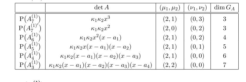
Table 1. The correspondence between the data that defines the linear problem and the q-Painlev´e equations. This data includes the determinant, and the asymptotic behavior of the solutions at x= 0 andx=∞in (3.1).
detA (µ1, µ2) (ν1, ν2) dimGA
P A(1)7
κ1κ2x3 (2,1) (0,3) 3
P A(1)7 ′
κ1κ2x2 (2,0) (0,2) 3
P A(1)6
κ1κ2x2(x−a1) (2,1) (0,2) 4
P A(1)5
κ1κ2x(x−a1)(x−a2) (2,1) (0,1) 5
P A(1)4
κ1κ2(x−a1)(x−a2)(x−a3) (2,1) (0,0) 6
P A(1)3
κ1κ2(x−a1)(x−a2)(x−a3)(x−a4) (2,2) (0,0) 7
4.1 q-P A(1)7
Let us consider the simplest case in a more precise manner than the others as a test case. The simplest q-difference case is the
{b0, b1:f, g} →
b0
q , b1q: ˜f ,˜g
,
where q=b0b1 and the evolution is
˜
f f = b1(1−g˜) ˜
g , ˜gg=
1
f, (4.1)
which is also known as q-PI. We note that this transformation gives us a copy of Z inside the
group of B¨acklund transformations [23]. We note that there exists also exists a Dynkin diagram automorphism in the group of B¨acklund transformations, however, we still do not know how these Dynkin diagram automorphisms manifest themselves in this theory. The associated linear problem, specified by Murata [17], is given by
Y(qx) =A(x)Y(x),
where
A(x) =
((x−y)(x−α) +z1)κ1 κ2w(x−y)
(xγ+δ)κ1
w (x−y+z2)κ2
.
We fix the determinant
detA(x) =κ1κ2x3,
and let A(0) possess one non-zero eigenvalue, λ1. This allows us to specify the values
α= λ1−z1κ1+ (y−z2)κ2
yκ1
, γ = (−2y−α+z2)κ2, δ = (yα+z1) (y−z2)κ2
y .
We make a choice of parameterization of z1 and z2, given by
z1= y2
z , z2=yz.
The problem possesses formal solutions aroundx= 0 and x=∞ specified by
The asymptotics of these solutions and the zeros of the determinant define the characteristic data to be
meaning our co-ordinate system for the A matrices should be
MA=
where we have the constraint
λ1λ2 =κ1κ2.
This specifies four parameters with one constraint, however, it is easy to verify on the level of parameters (and much more work to verify on the level of the Painlev´e variables) that
Tκ1,λ2 ◦T −1
κ1,λ1◦Tκ2,λ1 =Tκ1,λ2,
hence, we may regard Tκ1,λ2 as an element of the group generated by the other three elements.
Upon further examination, the action of Rκ1,κ2,λ1,λ2(x) = xI is represented by an identity on
the Painlev´e parameters, however, there is a q-shift of the asymptotic behaviors at 0 and ∞. We regard this as a trivial action,Tκ1,κ2,λ1,λ2, whereby, we have the relation
was that R(x) may be obtained directly from the solutions via expansions of
R(x) = ˜Y(x)Y(x)−1,
where Y =Y0 orY =Y∞. UsingY =Y0 an expansion of R(x) aroundx= 0 gives
where as usingY =Y∞ an expansion ofR around x=∞ gives the constant term gives
R(x) =
different for each case. Computing the compatibility condition for the two non-trivial generators gives the following relations
Tκ1,λ1 : ˜w=w
which is the lattice of connection preserving deformations.
We now specify the connection preserving deformation that definesq-PIas
q-PI:
which is decomposed elementary Schlesinger transformations q-PI = Tκ1,λ1 ◦T −1
. We choose but one element of infinite order that we are able to make a correspondence with, for this, in Sakai’s notation, we choose
s1◦σ(1357)(2460), which has the following effect
which is also known as q-P′
I. The surface corresponds to the same affine Weyl group as before,
however, the technical difference is that it corresponds to a copy of a root subsystem of E8(1)
where the lengths of the roots are different from those that correspond toq-P A(1)7
[23]. The associated linear problem forq-P A(1)7 ′
, has been given by Murata [17]. In terms of the theory presented above, the same theory applies in that the characteristic data is well defined, and the deformations are all prescribed in the same manner as forq-P A(1)7
. In short, we expect a three dimensional lattice of deformations as above. We take
A(x) =
and the choice of zis specified by
z1= y2
z , z2=z.
We find the solutions are given by
Y0(x) =
This allows us to specify the characteristic data to be
M =
and the defining co-ordinate system for A(x) to be
Tκ1,λ2 : ˜w=−qw y
z, yy˜ = λ1 qκ1
, zz˜ = λ1
qκ2 .
In a similar manner to the associated linear problem for P A(1)7
, we have
Z3 ∼=hTκ
1,λ1, Tκ1,λ2, Tκ1,κ2,λ1,λ2i=GA,
forming the lattice of connection preserving deformations. We now identify the evolution of q-P′
I as a decomposition into the basis for elementary
Schlesinger transformations above. q-P′
I=Tκ1,λ1◦T −1
κ1,λ2. The action is specified by
Tκ1,λ1 ◦T −1
κ1,λ2 : ˜w=w(1−z˜), yy˜ =
˜
z(qλ1−κ2z˜) qκ1(˜z−1)
, zz˜ = qκ1
κ2 y2,
where we may identify with the above evolutions as z=−1/g, y =√b0b1f and κ2b0 =q2λ1− q2κ
1.
4.3 q-P A(1)6
We now increase the dimension of the underlying lattice by introducing non-zero root of detA. We note that in accordance with the notation of Sakai [23], we chooseσ◦σto define the evolution of q-PII. This system may be equivalently written as
b0 b1 b2 :f, g
→
b0 b1 qb2 : ˜f ,˜g
,
where q=b0b1 and
˜
f f =− b2g˜ ˜
g+b1b2
, gg˜ =b1b2(1−f). (4.3)
We find a parameterization of the associated linear problem to be given by
A(x) =
κ1((x−α)(x−y) +z1) κ2w(x−y) κ1
w(γx+δ) κ2(x−y+z2)
!
,
where by letting
detA(x) =κ1κ2x2(x−a1),
we readily find the entries of A(x) are given by
α= −z1κ1+ (y−z2)κ2+λ1
yκ1
, γ =−2y−α+a1+z2, δ=
(yα+z1) (y−z2)
y .
We take a choice of z to be specified by
z1=
y(y−a1)
z , z2 =yz.
The formal symbolic solutions are specified by
Y0(x) =
−
w(1−z)
z−1 −wyκ2 1−z y(z−1)κ2−λ1
+O(x)
eq,λ1(x) 0
0 eq,λ2(x) θq(x)2
Y∞(x) =
and the zeros of detA(x) define the characteristic data to be
M =
This allows us to write co-ordinate system for A as
MA=
where we have the constraint
λ1λ2 =−a1κ1κ2.
For the same reasons as previous subsections, it suffices to defineTκ1,λ1,Tκ1,λ1 and Tκ1,κ2,λ1,λ2,
however, we also need to choose an element that changesa1. We chooseTa1,λ1, which is induced
by some Ra1,λ1. By solving the scalar determinantal problem, one arrives at the conclusion
detRa1,λ1 =
∞ we have the expansion
The full group of Schlesinger transformations is given by
Z4 ∼=hTa
1,λ1, Tκ1,λ1, Tκ1,λ2, Tκ1,κ2,λ1,λ2i=GA,
which is the lattice of connection preserving deformations. To obtain a full correspondence ofTa1,λ1 with (4.3) we let
y=a1f, z=−gb0 b2 ,
with the relations b0 = λ1 a1κ2
and b2 =− λ1 qa2
1κ1
. We know that the action of Ta1,λ1 ◦Tκ1,λ−12 is
trivial. I.e., we have
Ta1,λ1◦Tκ1,λ−12 : ˜w= κ1w
κ2
, y˜=qy, z˜=z,
which leaves f and g invariant. When we restrict our attention to f and g alone we only have a two dimensional lattice of transformations, corresponding to (A1+A1)(1).
4.4 q-P A(1)5
As a natural progression from the above cases, we allow two non-zero roots of the determinant. In doing so, we obtain an associated linear problem for bothq-PIIIandq-PIV. We also introduce
a symmetry as one is able to naturally permute the two roots of the determinant, which we will formalize later. We turn to the particular presentation of Noumi et al. [18]. We present a version of q-PIII as
b0 b1 b2 c :f, g
→
qb0 b1/q b2 c : ˜f ,˜g
,
where q=b0b1b2 and
˜
f = qc
f g
1 +gb0 g+b0
, ˜g= qc
2
gf˜
b1+qf˜ q+b1f˜ .
Using the same variables, a representation of q-PIV is given by
b0 b1 b2 c :f, g
→
b0 b1 b2 qc : ˜f ,g˜
,
where
˜
f f = c
2qb
1(1 +gb0+f gb1b0)b2 qb1b2c2+g+f gb1
, ˜gg= b0b1 q(gb0+ 1)b2c
2+f g
(gb0(f b1+ 1) + 1) .
These two equations are interesting as a pair as they have the same surface of initial conditions. If any natural correspondence was to be sought between the theory of the associated linear problems and the theory of the surfaces of initial conditions [23], these two equations should possess the same associated linear problem up to reparameterizations. It is interesting to note that the associated linear problems defined by [17] do indeed possess the same characteristic data and asymptotics. We unify them by writing them as one linear problem, given by
A(x) =
κ2((x−α)(x−y) +z1) κ2w(x−y) κ1
w(γx+δ) κ2(x−y+z2)
!
where
detA(x) =κ1κ2x(x−a1)(x−a2).
This determinant and allowing A(0) to have one non-zero eigenvalue, λ1, allows us to specify
the parameterization as
We choosez to be specified by
z1=
y(y−a1)
z , z2 =z(y−a2).
The formal solutions are given by
Y0(x) =
which is enough to define
M =
hence, the co-ordinates forA(x) may be stated as
MA=
We notice that there is a natural symmetry introduced in the parameterization, that is that A
is left invariant under the action
s1:
obtain the following correspondences:
We may now specify Ta2,λ1 =s1◦Ta1,λ1 ◦s1.
Ta2,λ1 : ˜w=w
1− qyκ1
zκ2
, y˜= qya1κ1+qzλ1
qyzκ1−z2κ2
, zz˜ = qyκ1(˜y−a1)
κ2(˜y−qa2) .
This gives us the full lattice
Z5 ∼=hTa
1,λ1, Ta2,λ1, Tκ1,λ1, Tκ1,λ2, Tκ1,κ2,λ1,λ2i=GA.
We identify the evolution ofq-PIII withTa1,λ1 under the change of variables
y= qb0b
2 1λ1 gκ2
, z=− f
qb1 ,
so long as the following relations hold:
b20 = a1
a2
, λ2 =c2κ2, κ2a2=−qb21λ1.
The symmetry between a1 and a2 alternates between the two translational components of the
lattice of translations.
With the above identification, we also deduceq-PVI may be identified with
Ta1,λ1◦Ta2,λ1◦Tκ1,λ2◦T −1
κ1,λ1: ˜w=w−
qw(y−a1)κ1 zκ2
, y˜= q(y−a1)λ1−qza1a2κ2
y(q(y−a1)κ1−zκ2) ,
˜
z=−qκ1(za1a2κ2+ (a1−y)λ1)
zκ2(a2(zκ2−qyκ1) +λ1) .
We also note that in addition toTκ1,κ2,λ1,λ2 being trivial, we have that according to the
variab-les f and g, the transformation Tκ
1,λ−11 ,a−11 ,a−12 =T −1
a1,λ1 ◦Tκ1,λ1◦T −1
a2,λ1 is also trivial.
4.5 q-P A(1)4
The next logical step in the progression of associated linear problems is to assume that the determinant has three non-zero roots. This brings us to the case of q-PV:
b0 b1 b2 b3 b4 :f, g
→
qb0 b1 b2 b3 b4/q : ˜f ,˜g
where
ff˜= b0+gb2
b0(gb2+ 1) (gb1b2+ 1)b3
, g˜g=
( ˜f−1)b0
˜
f b3−1
˜
f b2
˜
f b0b1b2b3−1
.
The associated linear problem was introduced by Murata [17], and the particular group has been explored in connection with the big q-Laguerre polynomials [20]. This case introduces two new symmetries; the first is that we have the symmetric group on the three roots of detA, and the other is that the two solutions at x = 0 are of the same order. The result is that they are interchangeable on the level of solutions of a single second order q-difference equation. The offshoot of this is, by including extra symmetries, we need only compute two non-trivial connection preserving deformations.
Let us proceed by first giving a parameterization of the associated linear problem. We let
A(x) =
κ1((x−α)(x−y) +z1) κ2w(x−y) κ1
w(γx+δ) κ2(x−y+z2)
!
where
detA(x) =κ1κ2(x−a1)(x−a2)(x−a3).
Differently to previous case, the determinant of A(0) is non-zero, hence, we require that the eigenvalues of A(0),λ1 andλ2, are both not necessarily zero. This determines that the
parame-ters inA(x) are specified by
where we choose our parameter z to be specified by
z1=
(y−a1) (y−a2)
z , z2=z(y−a3).
Our constraint is now
κ1κ2a1a2a3 =−λ1λ2.
The fundamental solutions are of the form
Y0(x) =
This specifies that our characteristic data may be taken to be
M =
and hence, our co-ordinate space forA(x) is given by
MA=
s1:
a1 a2 a3
κ1 κ2 λ1 λ2 :w, y, z
→
a2 a1 a3
κ1 κ2 λ1 λ2 :w, y, z
,
s2:
a1 a2 a3
κ1 κ2 λ1 λ2 :w, y, z
→
a1 a3 a2
κ1 κ2 λ1 λ2 :w, y, z y−a3 y−a2
.
If we now specify Tκ1,λ1, the trivial transformation, Tκ1,κ2,λ1,λ2 and Ta1,λ1, we may obtain a
ge-nerating set using the symmetries to obtain
Ta2,λ1 =s1◦Ta1,λ1 ◦s1, Ta3,λ1 =s2◦s1◦Ta1,λ1◦s1◦s2, Tκ1,λ2 =s0◦Tκ1,λ1 ◦s0.
The transformations Tκ1,λ1 and Ta1,λ1 are specified by the relations
Ta1,λ1 : ˜w=
w((y−a1)a2a3κ1κ2+ (qy(y−a1)κ1+z(a3−y)κ2)λ1) κ2((y−a1)a2a3κ1+z(a3−y)λ1)
,
˜
y=−a2(w−w˜) (qλ1+a3κ2z˜)
qλ1( ˜w+w(˜z−1)) ,
˜
z= zλ1(w−w˜) +a2κ1(w(y−a1) + (y(z−1) +a1) ˜w)
w(y−a1)a2κ1+wzλ1
,
Tκ1,λ1 : ˜w=
w −qκ1y2+ (q(a1+a2)κ1+zκ2)y−qa1a2κ1+qzλ1
yzκ1
,
˜
y= qλ1+a3κ2z˜
qψκ1λ1−qψκ1λ1z˜
, z˜= q(ψa1κ1−1) (ψa2κ1−1)
zψ(κ2+qψκ1λ1) ,
where we have introduced
ψ= y
a1a2κ1−zλ1 ,
for convenience. We may now identify the lattice of connection preserving deformations as
Z6 ∼=hTκ
1,λ1, Tκ1,λ2, Tκ1,κ2,λ1,λ2, Ta1,λ1, Ta2,λ1, Ta3,λ1i=GA.
We may identify the evolution of q-PV with the Schlesinger transformation
q-PV=Ta1,a2,λ1,λ2 : ˜w=w(1−z˜), yy˜ =
(qλ1+a3κ2z˜) (λ1z˜−qa1a2κ1) qκ1λ1(˜z−1)
,
˜
zz= q(y−a1) (y−a2)κ1 (y−a3)κ2
.
where the correspondence between y and z withf and g is given by
y= a2
f , z=− b2 b0
g,
under the relations
a1=a2b3, a2 =a3b4, qa2b0κ1 =−b2κ2, b0b1b4λ1 =a2κ2.
In addition toTκ1,κ2,λ1,λ2 being trivial, we also have that the transformationTa1,a2,a3,κ−11 ,λ1,λ2 is
4.6 q-P A(1)3
This particular case was originally the subject of the article by Jimbo and Sakai [14], which in-troduced the idea of the preservation of a connection matrix [3]. The article was also responsible for introducing a discrete analogue of the sixth Painlev´e equation [14], given by
b1 b2 b3 b4 b5 b6 b7 b8 :f, g
→
qb1 qb2 b3 b4 qb5 qb6 b7 b8 : ˜f ,˜g
,
where
˜
f f b7b8
= ˜g−qb1 ˜
g−b3
˜
g−qb2
˜
g−b4
, gg˜ b3b4
= f −b5
f −b7 f−b6 f−b8
, (4.5)
where
q = b3b4b5b6
b1b2b7b8 .
The way in which q-PVI, orq-P A(1)3 , was derived by Jimbo and Sakai [14] mirrors the theory
that led to the formulation of PVI by Fuchs via the classical theory of monodromy preserving
deformations [9,8]. The associated linear problem originally derived by Jimbo and Sakai [14] is given by
A(x) =
κ1((x−y)(x−α) +z1) κ2w(x−y) κ1
w(γx+δ) κ2((x−y)(x−β) +z2)
!
,
where letting the eigenvalues of A(0) be λ1 and λ2, and the determinant of A(x) be
detA(x) =κ1κ2(x−a1)(x−a2)(x−a3)(x−a4),
leads to
α= −z1κ1−(y(−2y+a1+a2+a3+a4) +z2)κ2+λ1+λ2
y(κ1−κ2)
,
β = (y(−2y+a1+a2+a3+a4) +z1)κ1+z2κ2−λ1−λ2
y(κ1−κ2)
,
γ =y2+ 2(α+β)y+αβ−a2a3−(a2+a3)a4−a1(a2+a3+a4) +z1+z2,
δ =−(yα+z1) (yβ+z2)−a1a2a3a4
y .
We need to choose how to define z, which we take to be specified by
z1=
(y−a1) (y−a2)
z , z2=z(y−a3) (y−a4).
The theory regarding the existence and convergence of Y0(x) and Y∞(x) for this case, where
the asymptotics of the leading terms in the expansion of A(x) around x = 0 and x = ∞ are invertible, was determined very early by Birkhoff et al. [3]. In light of this, we solve for the first terms ofY0 andY∞ so that we may take the expansion to be
Y0(x) =
w((yα+z1)κ1−(yβ+z2)κ2+λ1−λ2)
w((yα+z1)κ1−(yβ+z2)κ2−λ1+λ2)
It is this parameterization in which we have a number of symmetries being introduced. We have the group of permutations on the ai generated by the elements
s1:
which are all elementary B¨acklund transformations, as is the elementary transformation swap-ping the eigenvalues/asymptotic behavior at x= 0, given by
s4:
To obtain the corresponding permutation of κ1 and κ2 we multiplyY(x) on the left by
R(x) =
in which the resulting transformation is most cleanly represented in terms of the parameteriza-tion of the linear problem, given as
where
ψ= y(zκ2−qκ1)
q(a1a2κ1−zλ1) .
The remaining elementary Schlesinger transformations are obtained from the symmetries and the above shifts. This gives
Z7 ∼=hTκ
1,κ2,λ1,λ2, Tκ1,λ1, Tκ1,λ2, Ta1,λ1, Ta2,λ1, Ta3,λ1, Ta4,λ1i=GA.
We may identify the evolution ofq-PVI with the connection preserving deformation
q-PVI:
a1 a2 a3 a4
κ1 κ2 λ1 λ2 :w, y, z
→
qa1 qa2 a3 a4
κ1 κ2 qλ2 qλ1 : ˜w,y,˜ z˜
,
or in terms of Schlesinger transformations
q-PVI=Ta1,λ1,a2,λ2 : ˜w=
qwκ1(˜z−1) κ2z˜−qκ1
, yy˜ =−(a3a4κ2z˜−qλ1) (λ1z˜−qa1a2κ1)
λ1(˜z−1) (qκ1−κ2z˜) ,
˜
zz = q(y−a1) (y−a2)κ1 (y−a3) (y−a4)κ2
.
We make a the correspondence with (4.5) by letting y = f and z = g/b3, and the relations
between parameters are given by
a1=b5, a2=b6, a3 =b7, a4 =b8, κ1 = b4λ1 b2b7b8
, κ1= b3λ1 b2b7b8
,
which completes the correspondences. We remark that in the representation of (4.5) the trans-formation b5 →qb5, b6 → qb6,b7 → qb7, b8 → qb8 and f → qf is a trivial transformation and
corresponds to Ta1,a2,a3,a4,λ2
1,λ22, which may also be regarded as trivial.
5
Conclusion and discussion
The above list comprises of 2×2 associated linear problems forq-Painlev´e equations in which the associated linear problem is quadratic inx. The way in which we have increased the dimension of the underlying lattice of connection preserving deformations has been to successively increase the number of non-zero roots of the determinant. If we were to consider a natural extension of the q-P A(1)3
case by adding a root making the determinant of order five in x then we would necessarily obtain a matrix characteristically different from the Lax pair of Sakai [25] and Yamada [31]. Sakai adjoins two roots of the determinant while introducing a relation between κ1 and κ2 while Yamada [31] introduces four roots on top of the q-P A(1)3 case and
fixes the asymptotic behaviors atx = 0 andx=∞. This seems to skip the cases in which the determinant of A is five. Of course, the above theory could be applied to those Lax pairs of Sakai and Yamada [25,31], yet, the jump between the given characteristic data for the associated linear problems ofq-P A(1)3
andq-P A(1)2
expect a framework which gives rise to a lift of the entire group of B¨acklund transformations to the level of Schlesinger transformations. This work, and the work of Yamada [31] may provide valuable insight into this.
We note the exceptional work of Noumi and Yamada in this case for a continuous analogue in their treatment of PVI [19]. They are able to extend the work of Jimbo and Miwa [11]
for PVI in a manner that includes all the symmetries of PVI. We remark however that the
more geometric approach to Lax pairs explored by Yamada [32] gives us a greater insight into a possible fundamental link between the geometry and Lax integrability of the discrete Painlev´e equations.
References
[1] Adams R.C., On the linear ordinaryq-difference equation,Ann. of Math.30(1928), 195–205.
[2] Bellon M.P., Viallet C.-M., Algebraic entropy,Comm. Math. Phys.204(1999), 425–437,chao-dyn/9805006.
[3] Birkhoff G.D., General theory of linear difference equations,Trans. Amer. Math. Soc.12(1911), 243–284.
[4] Birkhoff G.D., The generalized Riemann problem for linear differential equations and the allied problems for linear difference andq-difference equations,Proc. Amer. Acad.49(1913), 512–568.
[5] Birkhoff G.D., Guenther P.E., Note on a canonical form for the linearq-difference system,Proc. Nat. Acad. Sci. USA27(1941), 218–222.
[6] Carmichael R.D., The general theory of linearq-difference equations,Amer. J. Math.34(1912), 147–168.
[7] Di Vizio L., Ramis J.-P., Sauloy J., Zhang C., ´Equations auxq-diff´erences,Gaz. Math.96(2003), 20–49.
[8] Fuchs R., ¨Uber lineare homogene Differentialgleichungen zweiter Ordnung mit drei im Endlichen gelegenen wesentlich singul¨aren Stellen,Math. Ann.63(1907), 301–321.
[9] Fuchs R., ¨Uber lineare homogene Differentialgleichungen zweiter Ordnung mit drei im Endlichen gelegenen wesentlich singul¨aren Stellen,Math. Ann.70(1911), 525–549.
[10] Gasper G., Rahman M., Basic hypergeometric series, Encyclopedia of Mathematics and its Applications,
Vol. 35, Cambridge University Press, Cambridge, 1990.
[11] Jimbo M., Miwa T., Monodromy preserving deformation of linear ordinary differential equations with ra-tional coefficients. II,Phys. D2(1981), 407–448.
[12] Jimbo M., Miwa T., Monodromy preserving deformation of linear ordinary differential equations with ra-tional coefficients. III,Phys. D4(1981), 26–46.
[13] Jimbo M., Miwa T., Ueno K., Monodromy preserving deformation of linear ordinary differential equations with rational coefficients. I. General theory andτ-function,Phys. D2(1981), 306–352.
[14] Jimbo M., Sakai H., A q-analog of the sixth Painlev´e equation, Lett. Math. Phys. 38 (1996), 145–154,
chao-dyn/9507010.
[15] Joshi N., Burtonclay D., Halburd R.G., Nonlinear nonautonomous discrete dynamical systems from a general
discrete isomonodromy problem,Lett. Math. Phys.26(1992), 123–131.
[16] Le Caine J., The linearq-difference equation of the second order,Amer. J. Math.65(1943), 585–600.
[17] Murata M., Lax forms of theq-Painlev´e equations, J. Phys. A: Math. Theor.42(2009), 115201, 17 pages,
arXiv:0810.0058.
[18] Noumi M., An introduction to birational Weyl group actions, in Symmetric Functions 2001: Surveys of
Developments and Perspectives, NATO Sci. Ser. II Math. Phys. Chem., Vol. 74, Kluwer Acad. Publ.,
Dordrecht, 2002, 179–222.
[19] Noumi M., Yamada Y., A new Lax pair for the sixth Painlev´e equation associated withsob(8), inMicrolocal Analysis and Complex Fourier Analysis, World Sci. Publ., River Edge, NJ, 2002, 238–252,math-ph/0203029.
[20] Ormerod C.M., A study of the associated linear problem forq-PV,arXiv:0911.5552.
[21] Papageorgiou V.G., Nijhoff F.W., Grammaticos B., Ramani A., Isomonodromic deformation problems for discrete analogues of Painlev´e equations,Phys. Lett. A164(1992), 57–64.
[22] Ramani A., Grammaticos B., Hietarinta J., Discrete versions of the Painlev´e equations,Phys. Rev. Lett.67
[23] Sakai H., Rational surfaces associated with affine root systems and geometry of the Painlev´e equations,
Comm. Math. Phys.220(2001), 165–229.
[24] Sakai H., Aq-analog of the Garnier system,Funkcial. Ekvac.48(2005), 273–297.
[25] Sakai H., Lax form of theq-Painlev´e equation associated with theA(1)2 surface,J. Phys. A: Math. Gen.39
(2006), 12203–12210.
[26] Sauloy J., Galois theory of Fuchsian q-difference equations, Ann. Sci. ´Ecole Norm. Sup. (4)36 (2003),
925–968,math.QA/0210221.
[27] Shioda T., Takano K., On some Hamiltonian structures of Painlev´e systems. I,Funkcial. Ekvac.40(1997),
271–291.
[28] Trjitzinsky W.J., Analytic theory of linearq-difference equations,Acta Math.61(1933), 1–38.
[29] van der Put M., Reversat M., Galois theory of q-difference equations,Ann. Fac. Sci. Toulouse Math. (6)
16(2007), 665–718,math.QA/0507098.
[30] van der Put M., Singer M.F., Galois theory of difference equations,Lecture Notes in Mathematics, Vol. 1666, Springer-Verlag, Berlin, 1997.
[31] Yamada Y., Lax formalism forq-Painlev´e equations with affine Weyl group symmetry of type En(1), Int.
Math. Res. Not., to appear,arXiv:1004.1687.
[32] Yamada Y., A Lax formalism for the elliptic difference Painlev´e equation,SIGMA5(2009), 042, 15 pages,
![Figure 1.This diagram represents the degeneration diagram for the surfaces of initial conditions ofmultiplicative type [23].](https://thumb-ap.123doks.com/thumbv2/123dok/914158.900807/6.612.112.515.455.533/figure-diagram-represents-degeneration-diagram-surfaces-conditions-ofmultiplicative.webp)