On Numerical Approximation
of an Optimal Control Problem
in Linear Elasticity
Sobre la Aproximaci´
on Num´
erica de un Problema
de Control ´
Optimo en Elasticidad Lineal
A. Rincon, (
[email protected]
)
I-Shih Liu, (
[email protected]
)
Instituto de Matem´atica, Universidade Federal do Rio de Janeiro
Caixa Postal 68530, Rio de Janeiro 21945-970, Brazil
Abstract
We apply the optimal control theory to a linear elasticity problem. It can be formulated as a minimization problem of a cost functional. Numerical approximations are based on the optimality system of the corresponding minimization problem. An iterative method is consid-ered, for which convergence of the approximate solutions is proved pro-vided that a penalization parameter in the cost functional is not too small. Numerical solutions are presented to emphasize the role of this parameter. It is shown that the iterative method suffers a drawback that the approximate solutions are not good enough because the penal-ization parameter can not be taken sufficiently small. Such a limitation on the parameter is not inherited from the use of a penalization param-eter in the cost functional. Indeed, some methods may be free of such a limitation. We have shown by a simple spectral analysis that the so-lution exists as the parameter tends to zero by the use of eigenfunction representations.
Key words and phrases: Optimal control, Linear elasticity, finite element method, Iterative method, Eigenfunction expansion.
Resumen
Aplicamos la teor´ıa del control ´optimo a un problema de elasticidad lineal que puede ser formulado como un problema de minimizaci´on de una funcional de costo. Las aproximaciones num´ericas se basan en el sistema de optimalidad del correspondiente problema de minimizaci´on. Se considera un m´etodo iterativo para el cual se prueba la convergencia de las soluciones aproximadas suponiendo que un par´ametro de pena-lizaci´on en la funcional de costo no sea muy peque˜no. Se presentan soluciones num´ericas para enfatizar el rol de este par´ametro. Se mues-tra que el m´etodo iterativo tiene el inconveniente de que las soluciones aproximadas no son suficientemente buenas porque el par´ametro de pe-nalizaci´on no puede ser tomado suficientemente peque˜no. Tal limitaci´on sobre el par´ametro no es heredada del uso de un par´ametro de penaliza-ci´on en la funcional de costo. En verdad, algunos m´etodos pueden estar libres de esa limitaci´on. Hemos mostrado mediante un simple an´alisis espectral que la soluci´on existe cuando el par´ametro tiende a cero me-diante el uso de representaciones con funciones propias.
Palabras y frases clave:Control ´optimo, elasticidad lineal, m´etodo de los elementos finitos, m´etodo iterativo, desarrollo en funciones propias.
1
Introduction
The theory of optimal control of systems governed by partial differential equa-tions was essentially developed by Lions [7]. Many different type of control problems have been considered and solutions by numerical methods have been widely studied in the literature (see for examples, [3, 5, 7, 8]).
Theory of optimal control governed by a scalar equation of elliptic type, such as those involving heat conduction, are well-known in the literature. The problem is usually formulated as a minimization problem of a cost functional, involving a positive parameter for technical reasons. For the practical ob-jective of the optimal control solution this penalization parameter should be taken as small as possible.
hence the iterative method which does not allow the parameter to be arbitrary small may hardly be able to deliver a satisfactory optimal solution. However, this limitation seems to have been overlooked in many similar problems in the literature [5, 8, 10], where the convergence of the numerical solution is ensured by simply taking this parameter as 1 or a fixed convenient positive number using gradient type methods. Therefore apparently those results may suffer the same drawback as ours in this respect.
Such a limitation is not inherited from the use of penalization parameter in the cost functional. Indeed, there are methods free of such limitation when the parameter tends to zero. For this reason, we shall consider a spectral analysis in which an explicit solution of the optimality system in Fourier series expansion can be obtained in the limit as the parameter tends to zero. A bold-faced letter stands for a vector quantity and its components are represented by the corresponding normal letter with subindices ranging from 1 ton, the dimension of the physical space. The usual summation convention will be used to the component indices, i.e., the repeated component indices indicate a sum over its range from 1 to n.
2
An Optimal Control Problem in Elasticity
We consider the following boundary value problem of Dirichlet type in linear elasticity:
− ∂
∂xj
Cijkl
∂uk
∂xl
=fi, in Ω
ui= 0, on ∂Ω
(1)
where the elasticity tensorCijkl and the external forcefi are given functions
of x = (xi) in a smooth region Ω ⊂ Rn with smooth boundary ∂Ω. The
problem is to determine the displacement fieldu= (ui) satisfying the system
(1). It is usually assumed that ([2])
a) The elasticity tensor Cijkl satisfy the condition:
Cijkl=Cjikl =Cijlk=Cklij. (2)
b) There are positive constantsCand ¯C, such that for any symmetric matrices
Sij,
CSijSij ≤CijklSijSkl≤CS¯ ijSij. (3)
By virtue of these assumptions, the bilinear functionσdefined by
σ(u,v) =
Z
Ω
Cijkl∂ui
∂xj
∂vk
∂xl
dx, ∀u,v∈(H01(Ω))n (4)
is an inner product in (H1
0(Ω))n, called the energy inner product. The energy
normkukσ=σ(u,u)1/2is equivalent to the standard normkuk1of the space
(H1(Ω))n foru∈(H1
0(Ω))n. Indeed, from (3) we have
Ckuk1≤ kukσ≤C¯kuk1. (5)
We denote the inner product in (L2(Ω))n by
(u,v)0= Z
Ω
u·vdv, ∀u,v ∈(L2(Ω))n,
where u·v = uivi is the usual inner product in Rn. The usual norm in
(L2(Ω))n will be denoted bykuk
0= (u,u) 1/2 0 .
The weak form of the problem (1) can now be stated as follows: For a given functionf ∈(L2(Ω))n, find the solutionu∈(H1
0(Ω))n such that
σ(u,v) = (f,v)0, ∀v ∈(H01(Ω))
n. (6)
We can verify easily that the bilinear functionσ(·) is continuous and coercive in (H1
0(Ω))n. Therefore, according to Lax-Milgram Theorem ([2, 9]) and by
the use of elliptical regularity, for anyf ∈(L2(Ω))n, there is a unique solution u∈(H1
0(Ω))n∩(H2(Ω))n. The unique solution for the givenf will be denoted
byu(f).
Now let us turn to the formulation of an optimal control problem to obtain a prescribed displacement by means of externally applied forces on the body. Suppose that the equilibrium position of the body has some prescribed form given by a function zo(x) ∈(L2(Ω))n, called an objective function. We can
ask the question of how to determine the functionf such thatu(f) is as close to the objective functionzo as possible in (L2(Ω))n.
By introducing thecost functionaldefined by
J(f) =ku(f)−zok2
0+Nkfk20, (7)
Determine a functiong∈Uadsuch that
J(g) = inf
J(f); f ∈Uad , (8)
where Uadis a convex and closed set of(L2(Ω))n.
The real goal of the problem is to minimize the first term of the cost functional. The second term is added to limit the cost of control. The non-negative penalty parameter N is used to change the relative importance of the two terms in the cost functional. Therefore, for real purpose in obtaining the optimal result, the constantN should be taken as small as possible.
3
Optimality System
For numerical calculation of the optimal control we shall establish a more convenient formulation in terms of a system of differential equations. By the use of the Gateaux-differential of the cost functionalJ, the problem (8) can be characterized by
Z
Ω
(u(g)−zo)·(u(v)−u(g))dx+N
Z
Ω
g·(v−g)dx≥0, ∀v∈Uad. (9)
In order to obtain a more convenient form for the numerical calculation of the functiong, we shall reformulate the problem through the adjoint system. Let the operator defined on the left hand side of the system (1) be denoted byA: (H1
0(Ω))n →(L2(Ω))n,
Aui=−
∂ ∂xj
Cijkl
∂uk
∂xl
. (10)
Since by assumption, the elasticity Cijkl is symmetric, the operatorAis
self-adjoint,i.e.,
(Au,v)0= (u, Av)0, ∀u,v∈(H01(Ω)) n.
If we define the adjoint system by
Ap=u(g)−zo in Ω,
p= 0 on ∂Ω, (11)
then by substituting (u(g)−zo) from (11) into (9), we have Z
Ω
Ap·(u(v)−u(g)) +N
Z
Ω
Since Ais self-adjoint andAu(f) =f from the system (1), we have
Z
Ω
(p+Ng)·(v−g)dx≥0, ∀v ∈Uad. (12)
We consider the case Uad= (L2(Ω))n, for which it follows that
g=−1
Np.
Therefore, we can define the optimality systemby
Au=−1
N p in Ω
Ap=u−zo in Ω
u=p= 0 on ∂Ω.
(13)
This is a coupled system, besides some other solving methods, such as conjugate gradient method, least-squared method [5, 10, 4], we shall consider an iterative method which uncouples the system.
4
Iterative Method
In order to get a numerical solution for the problem, the optimality system is uncoupled in the following way: Givenp0= 0 then the values of umandpm
are iteratively calculated from the following algorithm:
Aum=−1 Npm−
1 in Ω,
Apm=um−zo in Ω,
um=pm= 0 on ∂Ω,
(14)
We shall prove in the following theorem that the algorithm above is convergent ifN is not too small.
Theorem 4.1. There exists a positive constantδ, such that forN > δ,
{pm,um} → {p,u}strongly in(H1
0(Ω))n∩(H2(Ω))n,
where panduare solutions of the optimality system (13).
Proof. With the notation,
from (13) and (14) we have
Taking inner product of the first equation withUmand the second withPm
and integrating over Ω, we obtain by the use of (4) after integration by parts,
σ(Um,Um) =−1
Taking the energy norm of (16) and (17), we get
kUmk2
In these relations we have used the elementary inequality,ab≤ 1 2(α a
2+b2/α),
whereαis real positive number. Since the normsk·kσandk·k1are equivalent
in (H1
In the second part of the above relations, we have used the Poincar´e inequality, where the constant Kdepends on Ω only. Hence we have
(2N C2−K)kUmk21≤KkP
two inequalities we obtain
kPmk2 1≤γkP
m−1
k2
where
regularity. The convergence of the sequence{Um} also follows in exactly the same argument.
To conclude the proof of the theorem, we need to determine the constants
αandNso that the conditionγ <1 is satisfied. Moreover, the value ofαwill be chosen in such a way that the lower bound for N is as small as possible. Sinceα > r/2, letα=r/2+εforε >0, then the conditionγ <1 is equivalent
Let the right hand side be denoted by δ, which takes its minimal value at
ε=r/2. With this choice, we haveα=rand
N > δ= r 2 1 +r
2, r= K
C2, (20)
which ensures the conditionγ <1 and the theorem is proved.⊓⊔
Remark. On the value ofδ:
By the assumptions (2) and (3) on the elasticity tensorCijkl, the elliptic
operator A defined in (10) is self-adjoint and positive definite. Hence by the spectral theorem, the eigenvectors of A form an orthonormal basis of the Hilbert space (H1
Hence, it follows from (5) that
In order words, the constant K in the Poincar´e inequality can be taken as ¯
C/λ1, and we arrive at an estimated value ofδ,
N > δ= C¯ 2C2λ
1
1 + C¯
C4λ2 1
.
In particular, forA=−∆, the Laplace operator, and Ω = (0,1)×(0,1), we haveC= ¯C= 1 andλ1= 2π2, hence the constantN can be chosen as small
as 0.0254 and since the above estimate is not optimal the lower limit ofδcan be even smaller than this value as we shall see in the numerical example later.
4.1
Finite Element Approximation
Let Vh be the finite dimensional subspace of (H1
0(Ω))n in the finite element
approximation with maximum mesh size h. The Galerkin formulation of the iterative problem (14) is given as follows:
Given z0 ∈(L2(Ω))n andp0
h = 0, find umh ∈Vh andpmh ∈Vh such that
for allvh∈Vh,
(
σ(umh,vh) = (F(pmh−1),vh)0,
σ(pm
h,vh) = (umh −zo,vh)0.
(22)
By employing finite element basis functions in Vh, (22) are systems of linear
algebraic equations.
In Theorem 1, we have proved for N > δ that the numerical solution
{um,pm} for uncoupled system (14) converges to the solution{u,p} of the optimality system. In the next theorem, we claim that the numerical solu-tion of system (22), {umh,pmh}, obtained by the finite element method also
converges to {u,p}.
Theorem 4.2. LetN > δ, then form→ ∞ andh→0,
{umh,pmh} −→ {u,p} in (H1
0(Ω))n∩(H 2(Ω))n,
where δis the constant defined in Theorem 4.1.
Sinceumandpmare solutions in (H1
0(Ω))n∩(H2(Ω))n of the optimality
5
Eigenfunction Expansion Method
In the previous section, we have proposed an iterative method for which the approximate solution {umh,phm} converges strongly to the solution {u,p} in (H1
0(Ω))n ∩(H2(Ω))n, provided that the constant N > δ, meaning, N is
not allowed to be arbitrary small. In our numerical calculations, we have found that such a restriction onN could be quite unsatisfactory in practical solutions. In order to find the solution of the optimality system free from such a restriction, in the following, we shall analyze the problem via the eigenfunction expansion method.
Since the operator A is positive-definite and self-adjoint defined in the Hilbert spaceH = (H1
0(Ω))n∩(H2(Ω))n. By the spectral theorem,H admits
a complete orthonormal basis of eigenfunctions {ϕm} of A and the corre-sponding eigenvaluesλmcan be arranged in ascending order,
0< λm≤λm+1, m= 1,2,3. . . .
Consequently,{u,p} ∈H can be expressed in an eigenfunction expansion of the form:
Substituting into the equation (13)1, we obtain
∞
Similarly, from the equation (13)2, we obtain
or
∞
X
m=1
pmλm−(um−zm)ϕm(x) = 0,
where zm are the Fourier coefficients in the eigenfunction expansion of the
given objective function z0∈(L2(Ω))n:
From (25) and (27), we obtain the Fourier coefficients um andpm,
um= zm
From these solutions we can easily see that when N →0 the function p(x) tends to zero, while the solution u(x) converges to the objective function
z0(x). Moreover, by (28) it follows that kuk0<kz0k0 for anyN >0.
On the other hand, the optimal controlg ∈(L2(Ω))n admits a
represen-tation in Fourier series, and sinceg=−p/N we obtain
g(x) =
which tends to the expected solution given by the eigenfunction expansion of
6
Numerical Results
For convenience, we shall consider the Laplace operator,A=−∆, in the unit square Ω = (0,1)×(0,1) as an example. Mathematically, it is a very special case of the linear elasticity operator, in which the components of the equilib-rium equation become independent of each other and the problem (1) can be regarded as two independent problems of scalar equations for the individual components. But for the purpose of examining the qualitative behavior of the optimal control solutions, our numerical calculation, both in finite element iterative approximation and in Fourier series expansion, will be illustrated for the case of Laplace operator. For more general elliptic operators or more gen-eral domains, eigenfunctions for spectral representations can be constructed numerically.
Since u = p = 0 on ∂Ω the eigenvalues and the eigenfunctions of the Laplace operator are well-known and they are given by
λmn= (n2+m2)π2, ϕmn= sinmπxsinnπy.
The objective function can then be represented by
z0(x, y) =
∞
X
m,n=1
zmnsinmπxsinnπy.
Substituting into (28) and (30), we have the approximation of the objective function,
u(x, y) = ∞
X
m,n=1
zmn
N(m2+n2)2π4+ 1sinmπxsinnπy,
and the function of optimal control,
g(x, y) = ∞
X
m,n=1
(m2+n2)π2z mn
N(m2+n2)2π4+ 1sinmπxsinnπy.
The exact solution of optimal control is then given by the function in the limit when N→0,
g(x, y) = ∞
X
m,n=1
0.08
0
1.0 0.5 0 0.5
0
Fig. 1. Objective functionz0(x, y)
5 0
1.0 0.5 0 0.5
0
Fig. 2. Exact optimal controlg(x, y)
0.01
0
1.0 0.5 0 0.5
0
0.25
0
1.0 0.5 0 0.5
0
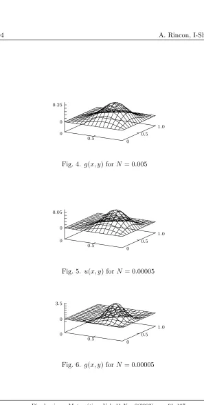
Fig. 4. g(x, y) forN = 0.005
0.05
0
1.0 0.5 0 0.5
0
Fig. 5. u(x, y) forN = 0.00005
3.5
0
1.0 0.5 0 0.5
0
0.08
0
1.0 0.5 0 0.5
0
Fig. 7. u(x, y) forN = 0
7
0
1.0 0.5 0 0.5
0
Fig. 8. g(x, y) forN = 0
For numerical calculations, we consider a prescribed objective function given by
z0(x, y) =16xy(1−x)(1−y)(x−y2)3.
In Fig. 1 and Fig. 2, the objective functionz0(x, y) and the exact optimal
control g(x, y) given above are shown. In finite element approximation, we have taken a mesh of 15×15 square elements. Remember that there is a lower limit of the parameterN. In the present case we have found that this limit is approximately equal to 5×10⁻³(Note that it is much smaller than the
that kuk0is much too small compared to the expected valuekz0k0.
On the other hand, there is no restriction on the value ofN for the method of Fourier series expansion. Approximation by Fourier series is calculated by a sum of 22 terms in eigenfunctionsϕmnform2+n2<62. Numerical solutions
are obtained for values ofN = 5×10⁻³, 5×10⁻⁵and also forN = 0. which
represents the exact solution to the problem. The figures for N = 5×10⁻³
are not shown here because they are practically identical to Figures 3 and 4 for the results of iterative approximation. Fig. 5, Fig. 6 and Fig. 7, Fig. 8 show the graphics for N = 5×10⁻⁵ andN = 0 respectively. We can see the
gradual improvement of the approximation for decreasing values ofN and an excellent agreement with the exact solutions shown in Fig. 1 and Fig. 2 for the case ofN = 0, for which the series are calculated with a finite sum of the first 22 terms only.
Acknowledgments: The author (ISL) acknowledges the partial support for research from CNPq of Brazil.
References
[1] Ciarlet, P. G.: The Finite Element Method for Elliptic Problems, North Holand, Amsterdam (1987).
[2] Fichera, G.: Existence Theorems in Elasticity, in Handbuch der Physik, Band VIa/2, Edited by C. Truesdell, Springer-Verlag (1972).
[3] Gill, S. I., Murray, W., Wright, M. H.: Practical Optimization, Academic Press (1988).
[4] Gunzburger, M. D.; Lee, H-C.: Analysis and approximation of optimal control problems for first-order elliptic systems in three dimensions. Appl. Math. Comput., 100, 49-70 (1999).
[5] Haslinger, J.; Neittaanm¨aki, P.: Finite Element Approximation for Opti-mal Shape Design: Theory and Applications, John Wiley & sons (1988).
[6] Kelley, C. T., Sachs, E. W.: Multilevel algorithms for constrained com-pact fixed point problems, SIAM J. Sci. Comput. 15, 645-667 (1994).
[8] Neittaanm¨aki, P., Tiba, D.: Optimal Control of Nonlinear Parabolic Sys-tems, Marcel Dekker, Inc. New York (1994).
[9] Oden, J. T., Reddy, J. N.: Variational Methods in Theoretical Mechanics, Spring-Verlag (1976).
[10] Pironneau, O.: Optimal Shape Design for Elliptic Systems, Springer-Verlag, Berlin (1984).