DIAGNOSTIC-ROBUST STATISTICAL ANALYSIS
FOR LOCAL SURFACE FITTING IN 3D POINT CLOUD DATA
Abdul Nurunnabi
a,*, David Belton
b, Geoff West
ba, b
Department of Spatial Sciences, Curtin University, Western Australia, Australia
a[email protected],
b{D.Belton, G.West}@curtin.edu.au
a,bCooperative Research Centre for Spatial Information
Commission III/4
KEY WORDS: 3D Modeling, Feature Extraction, Geometric Primitives, Laser Scanning, Local Normal Estimation, Photogrammetry, Plane Fitting, Surface Reconstruction
ABSTRACT:
This paper investigates the problem of local surface reconstruction and best fitting for planar surfaces from unorganized 3D point cloud data. Least Squares (LS), its equivalent Principal Component Analysis (PCA) and RANSAC are the three most popular techniques for fitting planar surfaces to 3D data. LS and PCA are sensitive to outliers and do not give reliable and robust parameter estimation. The RANSAC algorithm is robust but it is not completely free from the effect of outliers and is slow for large datasets. In this paper, we propose a diagnostic-robust statistical algorithm that uses both diagnostics and robust approaches in combination for fitting planar surfaces in the presence of outliers. Recently introduced high breakdown and fast Minimum Covariance Determinant (MCD) based location and scatter estimates are used for robust distance to identify outliers and a MCD based robust PCA approach is used as an outlier resistant technique for plane fitting. The benefits of the new diagnostic-robust algorithm are demonstrated with artificial and real laser scanning point cloud datasets. Results show that the proposed method is significantly better and more efficient than the other three methods for planar surface fitting. This method also has great potential for robust local normal estimation and for other surface shape fitting applications.
* Corresponding author.
1. INTRODUCTION
In many fields such as photogrammetry, reverse engineering and computational geometry, surface reconstruction and fitting for geometric primitives is a fundamental task with point cloud data. Much use is made of accurate local surface fitting and local normal estimation and the fact that these are related to each other. “In surface reconstruction, the quality of the approximation of the output surface depends on how well the estimated normals approximate the true normals of the sampled surface” (Tamal et al., 2005). Most man-made objects contain planar surfaces. Fitting a planar surface is closely related to local normal estimation for surface reconstruction, point cloud segmentation, classification and rendering (Schnabel et al., 2007; Pu et al., 2011). In fact, plane detection can be regarded as the first step in segmentation. In point cloud data analysis local normal estimation from a fitted local plane is used frequently (Hoppe et al., 1992; Wang et al., 2001). The Least Squares (LS) method, Principal Component Analysis (PCA) and RANdom Sample and Consensus (RANSAC) are the three most popular techniques for fitting planar surfaces to 3D data (Hoppe et al., 1992; Schnabel et al., 2007). Tarsha-Kurdi et al., (2007) show that the RANSAC is more efficient than the well-known Hough transform and note that the Hough-transform is very sensitive to the segmentation parameters values. Hence we compare RANSAC with our technique.
The majority of point cloud data is acquired by various measurement processes using a number of instruments
(sensors). The physical limitations of the sensors, boundaries between 3D features, occlusions, multiple reflectance and noise can produce off-surface points that appear to be outliers (Sotoodeh, 2006). Robust statistical approaches are regarded as one of the most effective solutions to the problems of outliers. Stewart (1999) states in his review paper: “It is important for the reader to note that robust estimators are not necessarily the only or even the best technique that can be used to solve the problems caused by outliers and multiple populations (structures) in all contexts”. The necessity of robust methods has been well described in the literature (e.g. Hampel et al., 1986). The goal of robust multivariate methods should be twofold: to identify outliers and to provide an analysis that has greatly reduced sensitivity to outliers. It is well-known that the LS and PCA methods are very sensitive to outliers and fail to reliably fit planes (Mitra and Nguyen, 2003). The RANSAC algorithm is not completely free from the effect of outliers and requires more processing time for large datasets. Moreover, “RANSAC is very efficient in detecting large planes in noisy point clouds but very slow to detect small planes in large point clouds” (Deschaud and Goulette, 2010). In this paper, we concentrate on planar surface fitting and local normal estimation of the fitted plane. Robust PCA often gives an accurate portrayal of the underlying data, but even so, it does not identify particular outliers that may be significant in their own right. To get more effective results, along with a robust version of PCA, it is important to have a complementary outlier identification method. We propose a new diagnostic-robust statistical technique for planar surface fitting in 3D point cloud
data, which is able to find outliers and robust estimates at the same time. We compare the new method with LS, PCA and RANSAC. The robustness of the methods is compared with respect to size of the data, outlier percentage and point density.
The remainder of the paper is arranged as follows: Section 2 briefly discusses the three related methods. In Section 3, we propose our technique for fitting planes and for local normal estimation from the best fitted plane. Section 4 contains results, and analyses the performance of the proposed technique through comparison with the other methods using simulated and real (mobile mapping laser scanning) datasets. Section 5 concludes the paper.
2. RELATED WORKS AND PRINCIPLES
In this section, we briefly discuss the basic notions of the related methods used in this paper.
2.1 Least Squares
The same basic principle of the LS method has been used in different ways for plane fitting. The principle is to minimize the sum of the squared residuals. Assume a sample of data points {pi (xi, yi , zi); i1,2,...,n} belong in a 3D point cloud and used to fit a plane. The plane equation is:
axbyczd0, (1)
where a, b, c and d are the parameters. The LS method is used to express the data points in the form (x,y,f(x,y)z) and to minimize the sum of squared residuals (r2),
z z i n
r n
i i i n
i
i min , 1,2,...,
1 2
1
2
(2)
where r is the distance between points and the fitted plane. The ith residual is a vertical distance and considered only in one (vertical) direction (z here) (Kwon et al., 2004). To overcome the bias to one direction, the approach of Total Least Squares (TLS) is proposed that minimizes the squared sum of the orthogonal distances between the points and the plane. In TLS, if the position (centre) of the plane is defined as c and n
is the unit normal to the plane, the parameters of the plane can be determined by solving:
n
p c n
i ni
T i n
cmin 1( ) , 1,2,...,
2 1
,
(3)
where p cT n i
)
( is the orthogonal distance between a plane and a point pi of the data. Hoppe et al., (1992) and later many use this idea for fitting a plane. The other way of parameter estimation is minimizing the orthogonal distance using the Singular Value Decomposition (SVD) of the data matrix.
2.2 Principal Component Analysis
PCA is a statistical technique that is typically used to identify a small set of mutually orthogonal variables which explain most of the underlying covariance structure of a dataset. Principal Components (PCs) are the linear combination of the original variables that rank the variability in the data through the variances, and produce the corresponding directions using the
eigenvectors of the covariance matrix. So, the first PC corresponds to the direction in which the projected observations have the largest variance, the second PC corresponds to the next direction and so on. Every PC describes a part of the data variance not explained by those with larger variances. Using only the top ranked PCs enable a reduced representation of the data. PCA minimizes the variance from the data by subtracting the mean from the corresponding variables and then performs SVD on that covariance matrix. This way PCA finds the required number of PCs. In the case of plane estimation, the first two PCs form a basis for the plane and the third PC is orthogonal to the first two and defines the normal of the fitted plane. Since the first two PCs explain the variability as much as possible with two dimensions, the fitted plane is the best 2D linear approximation to the data. Since the third PC expresses the least amount of variation, it can be used as the estimate of the coefficients of fitted plane. Hoppe et al., (1992) use the third PC as the normal of the plane. Later, many others use the PCA approach in different ways (Pauly et al., 2002) as an equivalent to LS. Although PCA is a powerful tool, it is well-known that the results are affected by anomalous observations.
2.3 RANSAC
The RANSAC algorithm, introduced by Fischler and Bolles (1981), extracts shapes and estimates the parameters of a model by randomly drawing a subset of data from the dataset. It is an iterative process consisting of two steps: hypothesize and test. First, a minimal subset (three points for a plane) is randomly selected and the required parameter estimation computed based on the subset. In the second step, the estimates are tested against all the data points to determine how many of them are consistent with the estimates. RANSAC divides data into inliers and outliers and yields parameters computed from the minimal set of inliers by using LS estimation with maximum support. It is conceptually simple, very general and can robustly deal with data containing more than 50% of outliers (Schnabel et al., 2007). Many authors use RANSAC for planar and local surface fitting (e.g., Schnabel et al., 2007). Since its inception, many versions of RANSAC (e.g., Torr and Zisserman, 2000; Michaelsen and Stilla, 2003) have been proposed. Torr and Zisserman (2000) point out that RANSAC can be sensitive to the choice of the correct noise threshold and when multiple model instances are present (see Zuliani, 2011). Schnabel et al., (2007) state that lack of efficiency and high memory consumption remain its major drawbacks.
3. PROPOSED ALGORITHM
The proposed Diagnostic-Robust PCA (DRPCA) algorithm is a combination of diagnostics and robust statistical techniques. First, we find candidate outliers using Robust Distance (RD). This reduces some outlier effects and makes the data more homogeneous. Second, we use robust PCA to find more candidate outliers, if any, and fit the plane in a robust way. The steps of the algorithm are:
i. calculate RD for the 3D point cloud,
ii. classify regular observations and outliers based on the RD, iii. perform robust PCA by using the regular observations from
step (ii),
iv. calculate orthogonal and score distances from step (iii), and classify the observations as outliers and regular observations by using orthogonal distance,
v. find the first three robust PCs based on the regular observations from step (iv), and
vi. fit a plane using the first two PCs from step (v) and find the third PC as the normal.
3.1 Robust Distance
In multivariate data, the distance of an observation from the centre of the data is not sufficient for outlier detection as the shape of the data has to be considered. The shape of multivariate data is quantified by the covariance structure of the data. The Mahalanobis Distance (MD) (Mahalanobis, 1936) is probably the most well-known distance measure that considers covariance in the variables. For a m-dimensional multivariate sample xi, MD is defined as:
MDi (xic)T1(xic), i1,2,...,n (4)
where c is the estimated arithmetic mean and ∑ is the covariance matrix of the sample data. “Although it is still quite easy to detect a single outlier by means of MD, this approach no longer suffices for multiple outliers because of the masking effect” (Rousseeuw and Driessen, 1999). Masking occurs when an outlying subset goes undetected because of the presence of another, usually adjacent, subset (Hadi and Simonoff, 1993). Hampel et al., (1986) point out that the MD is not robust because of the sensitivity of the mean and covariance matrix to outliers. It is necessary to use a distance that is based on robust estimators of multivariate location and scatter (Rousseeuw and Leroy, 2003). Many robust estimators have been introduced in the literature (see Maronna and Yohai, 1998). Minimum Covariance Determinant (MCD) is one of the most popular ones because it is computationally fast (Rousseeuw and Drissen, 1999). The MCD finds a subset of h
(
n/2) observations (out of n, the total number of observations) whose covariance matrix has the lowest determinant. The MCD estimate of location (cMCD) is then the average of the h points, and the MCD estimate of scatter (∑MCD) is the covariance matrix of the h points. The Robust Distance (RD) based on MCD is defined as:RDi (xicMCD)TMCD1 (xicMCD), i1,2,...,n. (5)
Rousseeuw and van Zomeren (1990) show that RD follows a Chi-square (χ2) distribution with m (number of variables) degrees of freedom and the observations that exceed √(χ2m,0.975) are identified as outliers.
3.2 Robust Principal Component Analysis
Generally, robust PCA is performed by computing the eigenvalues and eigenvectors of a robust estimator of the covariance or correlation matrix. A number of robust centre and covariance estimators have been introduced in the literature (e.g., M-estimators: see Maronna and Yohai, 1998; S-estimators: Rousseeuw and Leroy, 2003). Recently, Hubert and Rousseeuw (2005) introduce a new approach to robust PCA. The authors combine the idea of Projection Pursuit (PP) (Friedmann and Tukey, 1974) with the fast-MCD (Rousseeuw and Driessen, 1999). The PP is used to preprocess the data so that the transformed data are lying in a subspace whose dimension is at most n-1, and then the fast-MCD estimator is used to get the robust centre and covariance matrix. Reducing
the data space to the affine subspace spanned by the n
observations is especially useful when m n, but even when
m
n, the observations may span less than the wholem-dimensional space (Hubert and Rousseeuw, 2005). Since, “PP uses trimmed global measures; it has the advantage of robustness against outliers” (Friedman and Tukey, 1974). The fast-MCD contains time saving techniques; when n is large it fixes a lower number (500) of random subsets. Reduction of subsets has no effect because the algorithm uses outlyingness measure to use fewer subsets. In computation, first the data is compressed to the principal components defining potential directions. Then, each ith direction is scored by its corresponding value of outlyingness:
i n
v x
v x c v x
w T
i MCD
T i MCD T i
v
i , 1,2,...,
) (
) ( max
arg 1
(6)
where the maximum is overall directions, v is a univariate direction and xivTdenotes a projection of the ith observation on the direction v. On every direction a robust centre (cMCD) and scale (∑MCD) of the projected data points (xivT) is computed. Second, a fraction h (h should be greater than n/2; in this paper we use h=0.75n) of observations with the smallest values of wi are used to construct a robust covariance matrix ∑. Finally, robust PCA projects the data points onto the k-dimensional subspace spanned by the k (k=2 for plane fitting) largest eigenvectors (i.e., PCs) of the ∑ and computes their centre and shape by the re-weighted MCD. The eigenvectors of ∑ then determine the robust PCs.
While computing the robust PCA, we can flag outliers in a diagnostic way. Outliers can be two types: orthogonal outlier that lies away from the subspace spanned by the k principal components and is identified by a large Orthogonal Distance (OD), which is the distance between the observation (xi) and its projection (
x
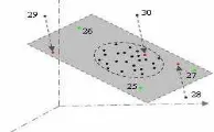
i) onto the k-dimensional PCA subspace. The other type of outlier is identified by the Score Distance (SD), which is measured within the PCA subspace. The cut-off value for the score distance is √(χ2k,0.975), and for the orthogonal distance is a scaled version of χ2 (see Hubert and Rousseeuw, 2005). We consider only the orthogonal outlier here because the points that are far away in terms of score should not be influential for plane fitting.Figure 1. Fitted plane, green points are distant in terms of score and red points are orthogonal outliers
In Figure 1, we see that the points 28, 29 and 30 (red points) are orthogonal outliers because they are away from the plane and distant by OD. Note that point 30 has low SD (projection is in the cluster) so would not be identified as an outlier without OD. Figure 1 shows clearly that points 25, 26 and 27 are in the plane although far from the main cluster of points, hence they are not considered as outliers. We use the remaining regular observations to get the final three PCs. The first two PCs are used for fitting the required plane and the third PC is considered as the estimated normal.
4. EXPERIMENTAL RESULTS and Zisserman, 2000) is an M-estimator based statistically robust version of RANSAC. We fit the planar surface and find normal and eigenvalues respective to the fitted plane. We calculate the bias angle (θ) (Figure 2 (a)) between the planes fitted to the data with and without outliers, defined by Wang et al., (2001) as:
with and without outliers respectively.
(a) (b)
Figure 2. (a) Bias angles (θ) between the fitted planes with and without outliers by different methods (b) variation along
the normal to the sample points
To compare results, we use the covariance technique and calculate the variation along the plane normal and the surface variation (see Pauly et al, 2002). Variation along the normal is defined by the corresponding eigenvalue (λ0) of the plane normal, and the surface variation at the point pi is defined as:
( ) , simulate the datasets for various sample sizes (n = 20, 50, 100 and 200) and outlier percentages (5, 10, 15, 20 and 25). We perform 1000 runs (for statistically representative results) for each and every sample size and outlier percentage. We compute the θ, λ0 and σp as the performance measures.
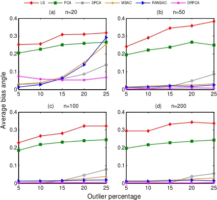
4.1.1 Bias angle: Figure 3 shows the average bias angles (in radians) for different sample sizes and outlier percentages. It shows the large difference between robust (RANSAC, MSAC, DPCA, DRPCA) and non-robust (LS, PCA) methods. LS is less consistent than PCA, and DRPCA has a lower bias angle than LS, PCA, DPCA, MSAC and RANSAC in most cases. Figure 3 (a), for sample size 20, shows that MSAC and RANSAC give inconsistent results for different percentages of outliers.
To show the effect of point density variation on bias angle, we create variations in surface directions (i.e., in x-y axes). We
5 10 15 20 25
Figure 3. Average bias angle versus outlier percentage for different sample sizes and outlier percentages
Variance I II III IV V
X (R,O) 3, 8 5, 10 7, 12 10, 15 15, 20 Y (R,O) 3, 0 5, 2 7, 4 10, 7 15, 12
Table 1. Variances for regular (R) and outlier (O) data
simulate 1000 sets of sample with 50 points in which 20% are outliers for different combinations of x, y variances. The rows of Table 1 show the variance combinations for regular (R) and outlier (O) data. Other criteria are the same as for the previous datasets. The results presented in Figure 4(a) show that robust methods are better than non-robust methods. Again the average bias angle for DRPCA is significantly less than for LS and PCA, and also better (less) than DPCA, MSAC and RANSAC.
It is known that surface thickness (roughness) influences surface fitting methods. To see the effect of roughness, we change the variance along the z (elevation) axis. Again we simulate 1000 datasets of 50 points with 20% outliers. The z
variances for regular observations are 0.001, 0.01, 0.02, 0.05, 0.1 and 0.2. The parameters for outliers (mean, variances for x,
y and z) are the same as for previous simulated datasets. Figure 4(b) shows that MSAC and RANSAC get worse compared to others with increasing z -variance.
I II III IV V
Variations in X-Y Variation s in Z
LS PCA DPCA MSAC RANSAC DRPCA
Figure 4. Average bias angle w.r.t. (a) point density variation (b) z variation
The above results in bias angle show that RANSAC performs better than MSAC in most of the cases, and DRPCA out performs DPCA. In the interests of brevity we do not consider DPCA and MSAC in the rest of the paper.
4.1.2 Surface variation: We simulate 1000 samples of 50 Median 4.85758 0.48155 0.00009 0.00006
λ0
Outliers 8 18 10 3
Mean 0.07405 0.01030 0.00001 0.00001 Median 0.07375 0.00992 0.00001 0.00001
σp methods. Every measure for DRPCA is better than for LS, PCA and the overall results are better than for RANSAC. In Figure 5, both the Box-plots show that DRPCA is better than classical PCA and competitive with RANSAC.
4.1.3 Performance time: Although DRPCA takes more time than LS and PCA to run, its computation time is still significantly less than for RANSAC. Table 3 shows the mean CPU time (in seconds) for various sample sizes (with 20% outliers) based on 1000 runs.
Sample size LS PCA RANSAC DRPCA
Table 3. Mean computation time
4.2 Real Point Cloud Data
We use laser scanner 3D data (Figure 6(a)) with 1,875 points. This dataset represents a saddle-back roof of a road side house; we consider it as a planar surface. Figures 6 (b) and 6 (c) show the points fitted by planes using LS and PCA showing that 15.9% outliers are detected by DRPCA and with the remaining regular points we fit the plane using robust PCA. Figure 6(g) shows there is no indication of outliers on that DRPCA plane.
Figure 6. (a) Real point cloud data (b) LS plane (c) PCA plane (d) outliers (red points) detected by RANSAC (e) RANSAC plane (f) red and blue points (outliers) detected by RD and OD
respectively (g) DRPCA plane
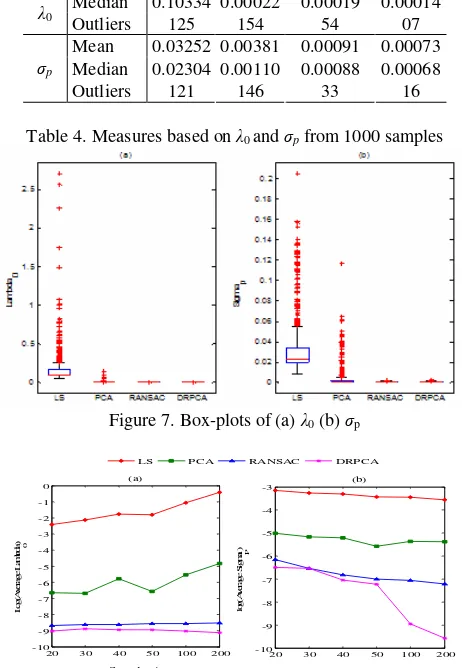
Considering the real dataset as a population, we take 1000 random samples of 50 points. We compute λ0 and σp values for LS, PCA, RANSAC and DRPCA. To illustrate the robustness of the methods, we draw Box-plots for λ0 and σp from the 1000 sampling results. Descriptive measures in Table 4 and Figure 7 show that non-robust techniques always perform worse than robust ones, and between the robust techniques DRPCA is better than RANSAC. For both λ0 and σp, DRPCA has the least number of outlying results. In the case of λ0, RANSAC fails 54 times whereas DRPCA fails only 7 times for 1000 runs.
Measures LS PCA RANSAC DRPCA
Mean 0.16525 0.00142 0.00019 0.00016 Median 0.10334 0.00022 0.00019 0.00014
λ0
Outliers 125 154 54 07
Mean 0.03252 0.00381 0.00091 0.00073 Median 0.02304 0.00110 0.00088 0.00068
σp
To evaluate the impact of sample (neighborhood) size variation
on λ0 and σp , we take 1000 random samples for each of 20, 30, 40, 50, 100 and 200 points. We take log values on the average
of λ0 and σp to emphasise the difference among different methods. Figure 8 shows that DRPCA performs the best for all sample sizes with all the values for the measures, and gives more accurate results (less values) for both λ0 and σp.
5. CONCLUSION AND FUTURE WORK
This paper proposes a diagnostic-robust PCA algorithm for fitting planar surfaces. Experiments based on artificial and real laser scanning datasets show that the proposed technique outperforms classical methods and is competitive with RANSAC. It has more accurate and robust results than the other methods. It gives the lowest bias angle and least amount of surface variation from the best fitted plane. It is also faster than RANSAC. Apart from accurately fitting planes in the presence of outliers, DRPCA can also generate accurate local surface normals. The technique has great potential for local surface estimation and geometric primitives fitting. Similar to many other robust techniques, it is not suitable for more than 50% of outliers. Future research will investigate its potential use for different feature extraction, estimation and fitting tasks.
ACKNOWLEDGEMENTS
This study has been carried out as a PhD research supported by a Curtin University International Postgraduate Research Scholarship (IPRS). The work has been supported by the Cooperative Research Centre for Spatial Information, whose activities are funded by the Australian Commonwealth's Cooperative Research Centres Programme. We are thankful to McMullen Nolan and Partners Surveyors for the real point cloud dataset. We also thank the anonymous reviewers for their constructive remarks.
REFERENCES
Deschaud, J. -E., and Goulette, F., 2010. A fast and accurate plane detection algorithm for large noisy point clouds using filtered normals and voxel growing. In Proc. Intl. Symp. 3DPVT, Paris.
Fischler, M. A., and Bolles, R. C., 1981. Random sample consensus: A paradigm for model fitting with applications to image analysis and automated cartography. Communications of the ACM, 24, pp. 381–395.
Friedman, J., and Tukey, J., 1974. A projection-pursuit algorithm for exploratory data analysis. IEEE Transaction on Computers, 23, pp. 881–889.
Hadi, A. S., and Simonoff, J. S., 1993. Procedures for the identification of outliers. JASA, 88, pp. 1264–1272.
Hampel, F., Ronchetti, E. Rousseeuw, P. J., and Stahel, W., 1986. Robust Statistics: The Approach Based on Influence Functions. John Wiley, New York.
Hoppe, H., De Rose, T., and Duchamp, T., 1992. Surface reconstruction from unorganized points. In Proc. of ACM SIGGRAPH, Vol. 26(2), pp. 71–78.
Hubert, M., and Rousseeuw, P. J., 2005. ROBPCA: A new approach to robust principal component analysis.
Technometrics, 47(1), pp. 64–79.
Kwon, S.-W., Bosche, F., Kim, C., Haas, C. T., and Liapi, K. A. 2004. Fitting range data to primitives for rapid local 3D modeling using sparse range point clouds. Automation in Construction, 13, pp. 67–81.
Mahalanobis, P. C., 1936. On the generalized distance in statistics. In Proc. of The ISI, Vol. 12, pp. 49–55.
Maronna, R. A., and Yohai, V., 1998. Robust estimation of multivariate location and scatter. Encyclopedia of Statistics, Vol. 2. John Wiley, New York.
Michaelsen, E., and Stilla, U., 2003. Good sample consensus estimation of 2D homographies for vehicle movement detection from thermal videos. In IAPRS, Vol. XXXIV/3, pp. 125–130.
Mitra, N. J., and Nguyen, A., 2003. Estimating surface normals in noisy point cloud data. 19th ACM Symposium on Computational Geometry, San Diego, California, pp. 322–328.
Pauly, M., Gross M., and Kobbelt, L. P., 2002. Efficient simplification of point sample surface. In Proc. of the Conference on Visualization, Washington, D.C., pp. 163–170.
Pu, S., Rutzinger, M., Vosselman, G., and Elberink, S. O., 2011. Recognizing basic structures from mobile laser scanning data for road inventory studies. In Press, ISPRS Journal of Photogrammetry and Remote Sensing.
Rousseeuw, P. J., and Driessen, K. V., 1999. A fast algorithm for the minimum covariance determinant estimator.
Technometrics, 41(3), pp. 212–223.
Rousseeuw, P. J., and Leroy, A., 2003. Robust Regression and Outlier Detection. John Wiley, New York.
Rousseeuw, P. J., and van Zomeren, B. C., 1990. Unmasking multivariate outliers and leverage points. JASA, 85(411), pp. 633–639.
Schnabel, R., Wahl, R., and Klein, R., 2007. Efficient RANSAC for point-cloud shape detection. The Eurographics Association and Blackwell Publishing, pp.1–12.
Sotoodeh, S., 2006. Outlier detection in laser scanner point clouds. In IAPRS, Dresden, Vol. XXXVI/5, pp. 297–301.
Stewart, C. V., 1999. Robust parameter estimation in computer vision. SIAM Review, 41(3), pp. 513–537.
Tamal, D., Gang, L., and Sun, J., 2005. Normal estimation for point cloud: a comparison study for a voronoi based method.
Eurographics Symp. on Point-Based Graphics. , pp. 39–46.
Tarsha-Kurdi, F., Landes, T., and Grussenmeyer, P., 2007. Hough-transform and extended RANSAC algorithms for automatic detection of 3D building roof planes from LiDAR data. In IAPRS, Vol. XXXVI/3, pp. 407–412.
Torr, P. H. S., and Zisserman, A., 2000. MLESAC: A new robust estimator with application to estimating image geometry. Journal of Computer Vision and Image Understanding, 78(1), pp. 138–156.
Wang, C., Tanahashi, H., and Hirayu, H., 2001. Comparison of local plane fitting methods for range data. In IEEE Computer Society Conference, CVPR'1, Kauai, Vol. 1, pp. 663–669.
Zuliani, M., 2011. RANSAC for Dummies. Draft, http://vision.ece.ucsb.edu/~zuliani/Research/RANSAC/docs/R ANSAC4Dummies.pdf (accessed 25 November 2011).