P H YS I C S
P R I NC I PLES
WITH
APPL I CATIONS
D O U G L A S C . G I A N C O L I
S E V
E
NT H
ED I T I O N
Boston Columbus Indianapolis New York San Francisco Upper Saddle River
C
H
A
P
T
E
R
Quantum Mechanics
of Atoms
CHAPTER-OPENING QUESTION—Guess now!
The uncertainty principle states that
(a) no measurement can be perfect because it is technologically impossible to make perfect measuring instruments.
(b) it is impossible to measure exactly where a particle is, unless it is at rest. (c) it is impossible to simultaneously know both the position and the
momen-tum of a particle with complete certainty.
(d) a particle cannot actually have a completely certain value of momentum.
B
ohr’s model of the atom gave us a first (though rough) picture of what an atom is like. It proposed explanations for why there is emission and absorp-tion of light by atoms at only certain wavelengths. The wavelengths of the line spectra and the ionization energy for hydrogen (and one-electron ions) are in excellent agreement with experiment. But the Bohr model had important limitations. It was not able to predict line spectra for more complex atoms—atoms with more than one electron—not even for the neutral helium atom, which has only two electrons. Nor could it explain why emission lines, when viewed with great precision, consist of two or more very closely spaced lines (referred to as fine structure). The Bohr model also did not explain why some spectral lines were brighter than others. And it could not explain the bonding of atoms in molecules or in solids and liquids.From a theoretical point of view, too, the Bohr model was not satisfactory: it was a strange mixture of classical and quantum ideas. Moreover, the wave–particle duality was not really resolved.
803
CONTENTS28–1 Quantum Mechanics—
A New Theory
28–2 The Wave Function and Its Interpretation; the Double-Slit Experiment
28–3 The Heisenberg Uncertainty Principle
28–4 Philosophic Implications; Probability versus Determinism
28–5 Quantum-Mechanical View of Atoms
28–6 Quantum Mechanics of the Hydrogen Atom;
Quantum Numbers 28–7 Multielectron Atoms; the
Exclusion Principle 28–8 The Periodic Table of
Elements
*28–9 X-Ray Spectra and Atomic Number *28–10 Fluorescence and
Phosphorescence 28–11 Lasers
*28–12 Holography
28
A neon tube is a thin glass tube, moldable into various shapes, filled with neon (or other) gas that glows with a particular color when a current at high voltage passes through it. Gas atoms, excited to upper energy levels, jump down to lower energy levels and emit light (photons) whose wavelengths (color) are characteristic of the type of gas.
We mention these limitations of the Bohr model not to disparage it—for it was a landmark in the history of science. Rather, we mention them to show why, in the early 1920s, it became increasingly evident that a new, more comprehensive theory was needed. It was not long in coming. Less than two years after de Broglie gave us his matter–wave hypothesis, Erwin Schrödinger (1887–1961; Fig. 28–1) and Werner Heisenberg (1901–1976; Fig. 28–2) independently developed a new comprehensive theory.
28–1
Quantum Mechanics—A New Theory
The new theory, called quantum mechanics, has been extremely successful. It unifies the wave–particle duality into a single consistent theory and has success-fully dealt with the spectra emitted by complex atoms, even the fine details. It explains the relative brightness of spectral lines and how atoms form molecules. It is also a much more general theory that covers all quantum phenomena from blackbody radiation to atoms and molecules. It has explained a wide range of natural phenomena and from its predictions many new practical devices have become possible. Indeed, it has been so successful that it is accepted today by nearly all physicists as the fundamental theory underlying physical processes.
Quantum mechanics deals mainly with the microscopic world of atoms and light. But this new theory, when it is applied to macroscopic phenomena, must be able to produce the old classical laws. This, the correspondence principle(already mentioned in Section 27–12), is satisfied fully by quantum mechanics.
This doesn’t mean we should throw away classical theories such as Newton’s laws. In the everyday world, classical laws are far easier to apply and they give sufficiently accurate descriptions. But when we deal with high speeds, close to the speed of light, we must use the theory of relativity; and when we deal with the tiny world of the atom, we use quantum mechanics.
Although we won’t go into the detailed mathematics of quantum mechanics, we will discuss the main ideas and how they involve the wave and particle properties of matter to explain atomic structure and other applications.
28–2
The Wave Function and Its
Interpretation; the Double-Slit Experiment
The important properties of any wave are its wavelength, frequency, and ampli-tude. For an electromagnetic wave, the frequency (or wavelength) determines whether the light is in the visible spectrum or not, and if so, what color it is. We also have seen that the frequency is a measure of the energy of the corresponding photon, (Eq. 27–4). The amplitude or displacement of an electromagnetic wave at any point is the strength of the electric (or magnetic) field at that point, and is related to the intensity of the wave (the brightness of the light).E=hf
FIGURE 28–2 Werner Heisenberg (center) on Lake Como (Italy) with Enrico Fermi (left) and Wolfgang Pauli (right).
For material particles such as electrons, quantum mechanics relates the wavelength to momentum according to de Broglie’s formula, Eq. 27–8. But what corresponds to the amplitudeordisplacementof a matter wave? The ampli-tude of an electromagnetic wave is represented by the electric and magnetic fields, EandB. In quantum mechanics, this role is played by the wave function, which is given the symbol (the Greek capital letter psi, pronounced “sigh”). Thus represents the wave displacement, as a function of time and position, of a new kind of field which we might call a “matter” field or a matter wave.
To understand how to interpret the wave function we make an analogy with light using the wave–particle duality.
We saw in Chapter 11 that the intensity Iof any wave is proportional to the square of the amplitude. This holds true for light waves as well, as we saw in Chapter 22. That is,
whereEis the electric field strength. From the particlepoint of view, the intensity of a light beam (of given frequency) is proportional to the number of photons,N, that pass through a given area per unit time. The more photons there are, the greater the intensity. Thus
This proportion can be turned around so that we have
That is, the number of photons (striking a page of this book, say) is proportional to the square of the electric field strength.
If the light beam is very weak, only a few photons will be involved. Indeed, it is possible to “build up” a photograph in a camera using very weak light so the effect of photons arriving can be seen. If we are dealing with only one photon, the relationship above can be interpreted in a slightly different way. At any point, the square of the electric field strength is a measure of the probability that a photon will be at that location. At points where is large, there is a high probability the photon will be there; where is small, the probability is low.
We can interpret matter waves in the same way, as was first suggested by Max Born (1882–1970) in 1927. The wave function may vary in magnitude from point to point in space and time. If describes a collection of many electrons, then at any point will be proportional to the number of electrons expected to be found at that point. When dealing with small numbers of electrons we can’t make very exact predictions, so takes on the character of a probability. If which depends on time and position, represents a single electron (say, in an atom), then is interpreted like this: at a certain point in space and time represents the probability of finding the electron at the given position and time.Thus is
often referred to as the probability densityorprobability distribution.
Double-Slit Interference Experiment for Electrons
To understand this better, we take as a thought experiment the familiar double-slit experiment, and consider it both for light and for electrons.
Consider two slits whose size and separation are on the order of the wave-length of whatever we direct at them, either light or electrons, Fig. 28–3. We know very well what would happen in this case for light, since this is just Young’s double-slit experiment (Section 24–3): an interference pattern would be seen on the screen behind. If light were replaced by electrons with wavelength comparable to the slit size, they too would produce an interference pattern (recall Fig. 27–12). In the case of light, the pattern would be visible to the eye or could be recorded on film, semiconductor sensor, or screen. For electrons, a fluores-cent screen could be used (it glows where an electron strikes).
°2
°2
°2
°, °2
°2
°
°
E2
E2 E2
AN rE2B N r E2.
I r E2 r N. I r E2,
°,
° °
l = h兾p,
SECTION 28–2 The Wave Function and Its Interpretation; the Double-Slit Experiment
805
FIGURE 28–3 Parallel beam, of light or electrons, falls on two slits whose sizes are comparable to the wavelength. An interference pattern is observed.
Light or electrons
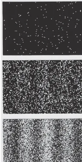
If we reduced the flow of electrons (or photons) so they passed through the slits one at a time, we would see a flash each time one struck the screen. At first, the flashes would seem random. Indeed, there is no way to predict just where any one electron would hit the screen. If we let the experiment run for a long time, and kept track of where each electron hit the screen, we would soon see a pattern emerging—the interference pattern predicted by the wave theory; see Fig. 28–4. Thus, although we could not predict where a given electron would strike the screen, we could predict probabilities. (The same can be said for photons.) The probability, as we saw, is proportional to Where is zero, we would get a minimum in the interference pattern. And where is a maximum, we would get a peak in the interference pattern.
The interference pattern would thus occur even when electrons (or photons) passed through the slits one at a time. So the interference pattern could not arise from the interaction of one electron with another. It is as if an electron passed through both slits at the same time, interfering with itself. This is possible because an electron is not precisely a particle. It is as much a wave as it is a particle, and a wave could travel through both slits at once. But what would happen if we covered one of the slits so we knew that the electron passed through the other slit, and a little later we covered the second slit so the electron had to have passed through the first slit? The result would be that no interference pattern would be seen. We would see, instead, two bright areas (or diffraction patterns) on the screen behind the slits.
If both slits are open, the screen shows an interference pattern as if each electron passed through both slits, like a wave. Yet each electron would make a tiny spot on the screen as if it were a particle.
The main point of this discussion is this: if we treat electrons (and other particles) as if they were waves, then represents the wave amplitude. If we treat them as particles, then we must treat them on a probabilistic basis. The square of the wave function, gives the probability of finding a given electron at a given point. We cannot predict—or even follow—the path of a single electron precisely through space and time.
28–3
The Heisenberg Uncertainty Principle
Whenever a measurement is made, some uncertainty is always involved. For example, you cannot make an absolutely exact measurement of the length of a table. Even with a measuring stick that has markings 1 mm apart, there will be an inaccuracy of perhaps or so. More precise instruments will produce more precise measurements. But there is always some uncertainty involved in a measurement, no matter how good the measuring device. We expect that by using more precise instruments, the uncertainty in a measurement can be made indefinitely small.
But according to quantum mechanics, there is actually a limit to the precision of certain measurements. This limit is not a restriction on how well instruments can be made; rather, it is inherent in nature. It is the result of two factors: the wave–particle duality, and the unavoidable interaction between the thing observed and the observing instrument. Let us look at this in more detail.
To make a measurement on an object without disturbing it, at least a little, is not possible. Consider trying to locate a lost Ping-pong ball in a dark room: you could probe about with your hand or a stick, or you could shine a light and detect the photons reflecting off the ball. When you search with your hand or a stick, you find the ball’s position when you touch it, but at the same time you unavoid-ably bump it, and give it some momentum. Thus you won’t know its future position. If you search for the Ping-pong ball using light, in order to “see” the ball at least one photon (really, quite a few) must scatter from it, and the reflected photon must enter your eye or some other detector. When a photon strikes an ordinary-sized object, it only slightly alters the motion or position of the object.
1 2mm
°2,
°
°2
°2
°2.
But a photon striking a tiny object like an electron transfers enough momentum to greatly change the electron’s motion and position in an unpredictable way. The mere act of measuring the position of an object at one time makes our knowledge of its future position imprecise.
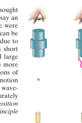
Now let us see where the wave–particle duality comes in. Imagine a thought experiment in which we are trying to measure the position of an object, say an electron, with photons, Fig. 28–5. (The arguments would be similar if we were using, instead, an electron microscope.) As we saw in Chapter 25, objects can be seen to a precision at best of about the wavelength of the radiation used due to diffraction. If we want a precise position measurement, we must use a short wavelength. But a short wavelength corresponds to high frequency and large
momentum and the more momentum the photons have, the more
momentum they can give the object when they strike it. If we use photons of longer wavelength, and correspondingly smaller momentum, the object’s motion when struck by the photons will not be affected as much. But the longer wave-length means lower resolution, so the object’s position will be less accurately known. Thus the act of observing produces an uncertainty in both the position and the momentumof the electron. This is the essence of the uncertainty principle first enunciated by Heisenberg in 1927.
Quantitatively, we can make an approximate calculation of the magnitude of the uncertainties. If we use light of wavelength the position can be measured at best to a precision of about That is, the uncertainty in the position measurement,
is approximately
Suppose that the object can be detected by a single photon. The photon has a momentum (Eq. 27–6). When the photon strikes our object, it will give some or all of this momentum to the object, Fig. 28–5. Therefore, the final xmomentum of our object will be uncertain in the amount
since we can’t tell how much momentum will be transferred. The product of these uncertainties is
The uncertainties could be larger than this, depending on the apparatus and the number of photons needed for detection. A more careful mathematical calcula-tion shows the product of the uncertainties as, at best, about
(28;1)
This is a mathematical statement of the Heisenberg uncertainty principle, or, as it is sometimes called, the indeterminancy principle. It tells us that we cannot measure both the position and momentum of an object precisely at the same time. The more accurately we try to measure the position, so that is small, the greater will be the uncertainty in momentum, If we try to measure the momentum very accurately, then the uncertainty in the position becomes large. The uncertainty principle does not forbid individual precise measurements, however. For example, in principle we could measure the position of an object exactly. But then its momentum would be completely unknown. Thus, although we might know the position of the object exactly at one instant, we could have no idea at all where it would be a moment later. The uncertainties expressed here are inherent in nature, and reflect the best precision theoretically attainable even with the best instruments.
¢p x.
¢x
(¢x)A¢pxB g h
2p
. (¢x)A¢pxB L (l)ah
lb L h.
¢px L h l
px = h兾l ¢x L l. ¢x,
l.
l, (p = h兾l);
SECTION 28–3 The Heisenberg Uncertainty Principle
807
UNCERTAINTY PRINCIPLE (position and momentum)
C A U T I O N
Uncertainties not due to instrument deficiency,
but inherent in nature (wave–particle)
FIGURE 28–5 Thought experiment for observing an electron with a powerful light microscope. At least one photon must scatter from the electron (transferring some momentum to it) and enter the microscope.
Electron
Light source
Light source
EXERCISE A Return to the Chapter-Opening Question, page 803, and answer it again now. Try to explain why you may have answered differently the first time.
Another useful form of the uncertainty principle relates energy and time, and we examine this as follows. The object to be detected has an uncertainty in position The photon that detects it travels with speed c, and it takes a
time to pass through the distance of uncertainty. Hence, the
measured time when our object is at a given position is uncertain by about
Since the photon can transfer some or all of its energy to our
object, the uncertainty in energy of our object as a result is
The product of these two uncertainties is
A more careful calculation gives
(28;2)
This form of the uncertainty principle tells us that the energy of an object can be uncertain (or can be interpreted as briefly nonconserved) by an amount for a time
The quantity appears so often in quantum mechanics that for conven-ience it is given the symbol (“h-bar”). That is,
By using this notation, Eqs. 28–1 and 28–2 for the uncertainty principle can be written
and
We have been discussing the position and velocity of an electron as if it were a particle. But it isn’t simply a particle. Indeed, we have the uncertainty principle because an electron—and matter in general—has wave as well as particle prop-erties. What the uncertainty principle really tells us is that if we insist on thinking of the electron as a particle, then there are certain limitations on this simplified view—namely, that the position and velocity cannot both be known precisely at the same time; and even that the electron does not havea precise position and momentum at the same time (because it is not simply a particle). Similarly, the energy can be uncertain (or nonconserved) by an amount for a time
Because Planck’s constant,h, is so small, the uncertainties expressed in the uncertainty principle are usually negligible on the macroscopic level. But at the level of atomic sizes, the uncertainties are significant. Because we consider ordinary objects to be made up of atoms containing nuclei and electrons, the uncertainty principle is relevant to our understanding of all of nature. The uncertainty principle expresses, perhaps most clearly, the probabilistic nature of quantum mechanics. It thus is often used as a basis for philosophic discussion.
¢t L U兾¢E. ¢E
(¢E)(¢t) g U.
(¢x)A¢p
xB g U
= 1.055 * 10–34J⭈s.
U = h
2p =
6.626 * 10–34J ⭈s 2p U
(h兾2p)
¢t L h兾(2p¢E).
¢E
(¢E)(¢t) g h
2p
. (¢E)(¢t) L ahc
l b a l
cb L h.
¢E L hc l
.
(= hf = hc兾l) ¢t L l
c.
¢t L ¢x兾c L l兾c ¢x L l.
Position uncertainty of electron. An electron moves in a
straight line with a constant speed which has been measured
to a precision of 0.10%. What is the maximum precision with which its position
could be simultaneously measured?
APPROACH The momentum is and the uncertainty in p is
The uncertainty principle (Eq. 28–1) gives us the smallest uncer-tainty in position using the equals sign.
SOLUTION The momentum of the electron is
The uncertainty in the momentum is 0.10%of this, or
From the uncertainty principle, the best simultaneous position measurement will have an uncertainty of
or 110 nm.
NOTE This is about 1000 times the diameter of an atom.
EXERCISE B An electron’s position is measured with a precision of Find the minimum uncertainty in its momentum and velocity.
Position uncertainty of a baseball. What is the uncertainty in position, imposed by the uncertainty principle, on a 150-g baseball thrown at
APPROACH The uncertainty in the speed is We multiply by m
to get and then use the uncertainty principle, solving for
SOLUTION The uncertainty in the momentum is
Hence the uncertainty in a position measurement could be as small as
NOTE This distance is far smaller than any we could imagine observing or measuring. It is trillions of trillions of times smaller than an atom. Indeed, the uncertainty principle sets no relevant limit on measurement for macroscopic objects.
lifetime calculated. The meson, discovered in 1974, was measured to have an average mass of (note
the use of energy units since ) and a mass “width” of By
this we mean that the masses of different mesons were actually measured to be slightly different from one another. This mass “width” is related to the very short lifetime of the before it decays into other particles. From the uncertainty principle, if the particle exists for only a time its mass (or rest energy) will
be uncertain by Estimate the lifetime.
APPROACH We use the energy–time version of the uncertainty principle,
Eq. 28–2.
SOLUTION The uncertainty of in the ’s mass is an uncertainty in
its rest energy, which in joules is
Then we expect its lifetime to be
Lifetimes this short are difficult to measure directly, and the assignment of very short lifetimes depends on this use of the uncertainty principle.
t L U
¢E =
1.055 * 10–34 J ⭈s
1.01 * 10–14 J L 1 * 10
–20 s.
t (= ¢t using Eq. 28–2) ¢E = A63 * 103 eVBA1.60 * 10–19 J兾eVB
= 1.01 * 10–14 J.
J兾c
63keV兾c2 J兾c ¢E L U兾¢t.
¢t,
J兾c
J兾c
63keV兾c2. E = mc2
3100MeV兾c2 J兾c
JⲐC EXAMPLE 28;3 ESTIMATE
¢x = U
¢p =
1.055 * 10–34 J⭈s
0.15kg⭈m兾s = 7 * 10
–34m.
¢p = m¢v = (0.150kg)(1m兾s) = 0.15kg⭈m兾s. ¢x. ¢p
¢v ¢v = 1m兾s.
(9362)mi兾h = (4261)m兾s? EXAMPLE 28;2
0.50 * 10–10m.
¢x L U
¢p =
1.055 * 10–34J ⭈s 1.0 * 10–27kg
⭈m兾s = 1.1
* 10–7 m,
¢p = 1.0* 10–27
kg⭈m兾s. p = mv = A9.11 * 10–31kgB A1.10 * 106m兾sB = 1.00 * 10–24kg⭈m兾s.
¢x ¢p = 0.0010p.
p = mv,
v = 1.10 *106 m兾s
EXAMPLE 28;1
28–4
Philosophic Implications;
Probability versus Determinism
The classical Newtonian view of the world is a deterministic one (see Section 5–8). One of its basic ideas is that once the position and velocity of an object are known at a particular time, its future position can be predicted if the forces on it are known. For example, if a stone is thrown a number of times with the same initial velocity and angle, and the forces on it remain the same, the path of the projectile will always be the same. If the forces are known (gravity and air resis-tance, if any), the stone’s path can be precisely predicted. This mechanistic view implies that the future unfolding of the universe, assumed to be made up of particulate objects, is completely determined.This classical deterministic view of the physical world has been radically altered by quantum mechanics. As we saw in the analysis of the double-slit experiment (Section 28–2), electrons all treated in the same way will not all end up in the same place. According to quantum mechanics, certain probabilities exist that an elec-tron will arrive at different points. This is very different from the classical view, in which the path of a particle is precisely predictable from the initial position and velocity and the forces exerted on it. According to quantum mechanics, the position and velocity of an object cannot even be known accurately at the same time. This is expressed in the uncertainty principle, and arises because basic entities, such as electrons, are not considered simply as particles: they have wave properties as well. Quantum mechanics allows us to calculate only the probability†that, say,
an electron (when thought of as a particle) will be observed at various places. Quantum mechanics says there is some inherent unpredictability in nature. This is very different from the deterministic view of classical mechanics.
Because matter is considered to be made up of atoms, even ordinary-sized objects are expected to be governed by probability, rather than by strict deter-minism. For example, quantum mechanics predicts a finite (but negligibly small) probability that when you throw a stone, its path might suddenly curve upward instead of following the downward-curved parabola of normal projectile motion. Quantum mechanics predicts with extremely high probability that ordinary objects will behave just as the classical laws of physics predict. But these predictions are considered probabilities, not absolute certainties. The reason that macroscopic objects behave in accordance with classical laws with such high probability is due to the large number of molecules involved: when large numbers of objects are present in a statistical situation, deviations from the average (or most probable) approach zero. It is the average configuration of vast numbers of molecules that follows the so-called fixed laws of classical physics with such high probability, and gives rise to an apparent “determinism.” Deviations from classical laws are observed when small numbers of molecules are dealt with. We can say, then, that although there are no precise deterministic laws in quantum mechanics, there are statistical laws based on probability.
It is important to note that there is a difference between the probability imposed by quantum mechanics and that used in the nineteenth century to understand thermodynamics and the behavior of gases in terms of molecules (Chapters 13 and 15). In thermodynamics, probability is used because there are far too many particles to keep track of. But the molecules are still assumed to move and interact in a deterministic way following Newton’s laws. Probability in quantum mechanics is quite different; it is seen as inherentin nature, and not as a limitation on our abilities to calculate or to measure.
r0 Nucleus
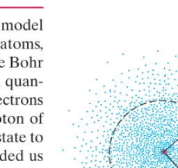
FIGURE 28–6 Electron cloud or “probability distribution” for the ground state of the hydrogen atom, as seen from afar. The dots represent a hypothetical detection of an electron at each point: dots closer together represent more probable presence of an electron (denser cloud). The dashed circle represents the Bohr radius r0.
The view presented here is the generally accepted one and is called the Copenhagen interpretationof quantum mechanics in honor of Niels Bohr’s home, since it was largely developed there through discussions between Bohr and other prominent physicists.
Because electrons are not simply particles, they cannot be thought of as following particular paths in space and time. This suggests that a description of matter in space and time may not be completely correct. This deep and far-reaching conclusion has been a lively topic of discussion among philosophers. Perhaps the most important and influential philosopher of quantum mechanics was Bohr. He argued that a space–time description of actual atoms and electrons is not possible. Yet a description of experiments on atoms or electrons must be given in terms of space and time and other concepts familiar to ordinary experience, such as waves and particles. We must not let our descriptionsof experiments lead us into believ-ing that atoms or electrons themselves actually move in space and time as classical particles.
28–5
Quantum-Mechanical View
of Atoms
At the beginning of this Chapter, we discussed the limitations of the Bohr model of atomic structure. Now we examine the quantum-mechanical theory of atoms, which is a far more complete theory than the old Bohr model. Although the Bohr model has been discarded as an accurate description of nature, nonetheless, quan-tum mechanics reaffirms certain aspects of the older theory, such as that electrons in an atom exist only in discrete states of definite energy, and that a photon of light is emitted (or absorbed) when an electron makes a transition from one state to another. But quantum mechanics is a much deeper theory, and has provided us with a very different view of the atom. According to quantum mechanics, electrons do not exist in well-defined circular orbits as in the Bohr model. Rather, the electron (because of its wave nature) can be thought of as spread out in space as a “cloud.” The size and shape of the electron cloud can be calculated for a given state of an atom. For the ground state in the hydrogen atom, the electron cloud is spherically symmetric, as shown in Fig. 28–6. The electron cloud at its higher densities roughly indicates the “size” of an atom. But just as a cloud may not have a distinct border, atoms do not have a precise boundary or a well-defined size. Not all electron clouds have a spherical shape, as we shall see later in this Chapter.
The electron cloud can be interpreted from either the particle or the wave viewpoint. Remember that by a particle we mean something that is localized in space—it has a definite position at any given instant. By contrast, a wave is spread out in space. The electron cloud, spread out in space as in Fig. 28–6, is a result of the wave nature of electrons. Electron clouds can also be interpreted as probability distributions (or probability density) for a particle. As we saw in Section 28–3, we cannot predict the path an electron will follow (thinking of it as a particle). After one measurement of its position we cannot predict exactly where it will be at a later time. We can only calculate the probability that it will be found at different points. If you were to make 500 different measurements of the position of an electron in a hydrogen atom, the majority of the results would show the electron at points where the probability is high (dark area in Fig. 28–6). Only occasionally would the electron be found where the probability is low. The electron cloud or probability distribution becomes small (or thin) at places, especially far away, but never becomes zero. So quantum mechanics suggests that an atom is notmostly empty space, and that there is no truly empty space in the universe.
28–6
Quantum Mechanics of the
Hydrogen Atom; Quantum Numbers
We now look more closely at what quantum mechanics tells us about the hydrogen atom. Much of what we say here also applies to more complex atoms, which are discussed in the next Section.Quantum mechanics is a much more sophisticated and successful theory than Bohr’s. Yet in a few details they agree. Quantum mechanics predicts the same basic energy levels (Fig. 27–29) for the hydrogen atom as does the Bohr model. That is,
wheren is an integer. In the simple Bohr model, there was only one quantum number,n. In quantum mechanics, four different quantum numbers are needed to specify each state in the atom:
(1) The quantum number, n, from the Bohr model is found also in quantum mechanics and is called the principal quantum number. It can have any integer value from 1 to The total energy of a state in the hydrogen atom depends on n, as we saw above.
(2) The orbital quantum number, is related to the magnitude of the angular momentum of the electron; can take on integer values from 0 to
For the ground state, can only be zero.†For can be 0, 1, or 2.
The actual magnitude of the angular momentum Lis related to the quantum number by
(28;3)
(where again ). The value of has almost no effect on the total energy in the hydrogen atom; only n does to any appreciable extent (but see fine structurebelow). In atoms with two or more electrons, the energy does depend on as well as n, as we shall see.
(3) The magnetic quantum number, is related to the directionof the electron’s angular momentum, and it can take on integer values ranging from to
For example, if then can be or Since angular
momentum is a vector, it is not surprising that both its magnitude and its direc-tion would be quantized. For the five different directions allowed can be represented by the diagram of Fig. 28–7. This limitation on the direction of is often called space quantization. In quantum mechanics, the direction of the angular momentum is usually specified by giving its component along the zaxis (this choice is arbitrary). Then is related to by the equation
The values of and are not definite, however. The name for derives not from theory (which relates it to ), but from experiment. It was found that when a gas-discharge tube was placed in a magnetic field, the spectral lines were split into several very closely spaced lines. This splitting, known as the Zeeman effect, implies that the energy levels must be split (Fig. 28–8), and thus that the energy of a state depends not only on nbut also on when a mag-netic field is applied—hence the name “magnetic quantum number.”
ml
†This replaces Bohr theory, which assigned to the ground state (Eq. 27 –11).
l=1
FIGURE 28–7 Quantization of angular momentum direction for
(Magnitude of is )
L = 16U.
LB
l = 2.
FIGURE 28–8 Energy levels (not to scale). When a magnetic field is applied, the energy level is split into five separate levels, corresponding to the five values of
An
level is split into three levels Transitions can occur between levels (not all transitions are shown), with photons of several slightly different frequencies being given off (the Zeeman effect).
(4) Finally, there is the spin quantum number, which for an electron can have
only two values, and The existence of this quantum
number did not come out of Schrödinger’s original wave theory, as didn, and Instead, a subsequent modification by P. A. M. Dirac (1902–1984) explained its presence as a relativistic effect. The first hint that was needed, however, came from experiment. A careful study of the spectral lines of hydrogen showed that each actually consisted of two (or more) very closely spaced lines even in the absence of an external magnetic field. It was at first hypothesized that this tiny splitting of energy levels, called fine structure, was due to angular momentum associated with a spinning of the electron. That is, the electron might spin on its axis as well as orbit the nucleus, just as the Earth spins on its axis as it orbits the Sun. The interaction between the tiny current of the spinning electron could then interact with the magnetic field due to the orbiting charge and cause the small observed splitting of energy levels. (The energy thus depends slightly on and )†Today we consider the picture of a spinning electron as
not legitimate. We cannot even view an electron as a localized object, much less a spinning one. What is important is that the electron can have two different states due to some intrinsic property that behaves like an angular momentum, and we still call this property “spin.” The two possible values of ( and ) are often said to be “spin up” and “spin down,” referring to the two possible directions of the spin angular momentum.
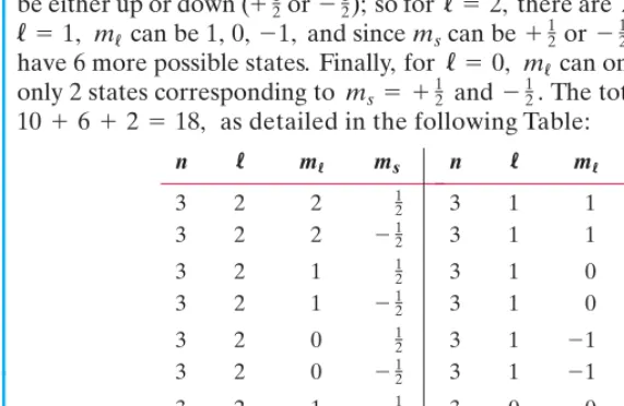
The possible values of the four quantum numbers for an electron in the hydrogen atom are summarized in Table 28–1.
–1 †Fine structure is said to be due to a spin–orbit interaction.
Possible states for How many dif-ferent states are possible for an electron with principal quantum number
RESPONSE For can have the values For can
be which is five different possibilities. For each of these, can
be either up or down ( or ); so for there are states. For
can be and since can be or for each of these, we
have 6 more possible states. Finally, for can only be 0, and there are only 2 states corresponding to and The total number of states is
as detailed in the following Table: 10 + 6 + 2 = 18,
CONCEPTUAL EXAMPLE 28;4
TABLE 28–1 Quantum Numbers for an Electron
Name Symbol Possible Values
Principal n
EXERCISE C An electron has Which of the following values of are possible: 4, 3, 2, 1, 0, –1,–2, –3, –4?
EandLfor Determine (a) the energy and (b) the orbital angular momentum for an electron in each of the hydrogen atom states with , as in Example 28–4.
APPROACH The energy of a state depends only on n, except for the very small
corrections mentioned above, which we will ignore. Energy is calculated as in the
Bohr model, For angular momentum we use Eq. 28–3.
SOLUTION (a) Since for all these states, they all have the same energy,
(b) For Eq. 28–3 gives
For
For
NOTE Atomic angular momenta are generally given as a multiple of ( or in this case), rather than in SI units.
EXERCISE D What are the energy and angular momentum of the electron in a hydrogen atom with
Although and do not significantly affect the energy levels in hydrogen, they do affect the electron probability distribution in space. For and can only be zero and the electron distribution is as shown in Fig. 28–6. For
can be 0 or 1. The distribution for is shown in Fig. 28–9a, and it is seen to differ from that for the ground state (Fig. 28–6), although it is still spherically symmetric. For the distributions are not spherically symmetric as shown in Figs. 28–9b (for ) and 28–9c (for or ). Although the spatial distributions of the electron can be calculated for the various states, it is difficult to measure them experimentally. Most of the experi-mental information about atoms has come from a careful examination of the emission spectra under various conditions as in Figs. 27–23 and 24–28.
[Chemists refer to atomic states, and especially the shape in space of their probability distributions, as orbitals. Each atomic orbital is characterized by its
quantum numbers n, and and can hold one or two electrons ( or
); s-orbitals are spherically symmetric, Figs. 28–6 and 28–9a; p-orbitals can be dumbbell shaped with lobes, Fig. 28–9b, or donut shaped
if combining and Fig. 28–9c.]
Selection Rules: Allowed and Forbidden Transitions
Another prediction of quantum mechanics is that when a photon is emitted or absorbed, transitions can occur only between states with values of that differ by exactly one unit:
According to this selection rule, an electron in an state can jump only to a
state with or It cannot jump to a state with or A
tran-sition such as to is called a forbidden transition. Actually, such a transition is not absolutely forbidden and can occur, but only with very low probability compared to allowed transitions—those that satisfy the selection rule Since the orbital angular momentum of an H atom must change by one unit when it emits a photon, conservation of angular momentum tells us that the photon must carry off angular momentum. Indeed, experimental evidence of many sorts shows that the photon can be assigned a spin angular momentum of 1U. ¢l = &1.
28–7
Multielectron Atoms;
the Exclusion Principle
We have discussed the hydrogen atom in detail because it is the simplest to deal with. Now we briefly discuss more complex atoms, those that contain more than one electron. Their energy levels can be determined experimentally from an analysis of their emission spectra. The energy levels are notthe same as in the H atom, because the electrons interact with each other as well as with the nucleus. Each electron in a complex atom still occupies a particular state characterized by the
quantum numbers n, and For atoms with more than one electron,
the energy levels depend on both nand
The number of electrons in a neutral atom is called its atomic number,Z; Zis also the number of positive charges (protons) in the nucleus, and determines what kind of atom it is. That is,Zdetermines the fundamental properties that dis-tinguish one type of atom from another.
To understand the possible arrangements of electrons in an atom, a new principle was needed. It was introduced by Wolfgang Pauli (1900–1958; Fig. 28–2) and is called the Pauli exclusion principle. It states:
No two electrons in an atom can occupy the same quantum state.
Thus, no two electrons in an atom can have exactly the same set of the quantum numbersn, and The Pauli exclusion principle forms the basis not only for understanding atoms, but also for understanding molecules and bonding, and other phenomena as well. (See also note at end of this Section.)
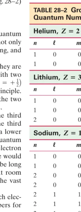
Let us now look at the structure of some of the simpler atoms when they are in the ground state. After hydrogen, the next simplest atom is heliumwith two electrons. Both electrons can have because one can have spin up
and the other spin down thus satisfying the exclusion principle. Since then and must be zero (Table 28–1, page 813). Thus the two electrons have the quantum numbers indicated at the top of Table 28–2.
Lithium has three electrons, two of which can have But the third cannot have without violating the exclusion principle. Hence the third
electron must have It happens that the level has a lower
energy than So the electrons in the ground state have the quantum numbers indicated in Table 28–2. The quantum numbers of the third electron
could also be, say, But the atom in this case would
be in an excited state, because it would have greater energy. It would not be long before it jumped to the ground state with the emission of a photon. At room temperature, unless extra energy is supplied (as in a discharge tube), the vast majority of atoms are in the ground state.
We can continue in this way to describe the quantum numbers of each elec-tron in the ground state of larger and larger atoms. The quantum numbers for sodium, with its eleven electrons, are shown in Table 28–2.
EXERCISE E Construct a Table of the ground-state quantum numbers for beryllium, (like those in Table 28–2).
Figure 28–10 shows a simple energy level diagram where occupied states are
shown as up or down arrows and possible empty states are
shown as a small circle. A
ms = ±
SECTION 28–7 Multielectron Atoms; the Exclusion Principle
815
TABLE 28–2 Ground-State
FIGURE 28–10 Energy level diagrams (not to scale) showing occupied states (arrows) and unoccupied states ( ) for the ground states of He, Li, and Na. Note that we have shown the
The ground-state configuration for all atoms is given in the Periodic Table, which is displayed inside the back cover of this book, and discussed in the next Section. [The exclusion principleapplies to identical particles whose spin quantum num-ber is a half-integer ( and so on), including electrons, protons, and neutrons; such particles are called fermions, after Enrico Fermi who derived a statistical theory describing them. A basic assumption is that all electrons are identical, indis-tinguishable one from another. Similarly, all protons are identical, all neutrons are identical, and so on. The exclusion principle does not apply to particles with integer spin (0, 1, 2, and so on), such as the photon and meson, all of which are referred to as bosons(after Satyendranath Bose, who derived a statistical theory for them).]
28–8
The Periodic Table of Elements
More than a century ago, Dmitri Mendeleev (1834–1907) arranged the (then) known elements into what we now call the Periodic Tableof the elements. The atoms were arranged according to increasing mass, but also so that elements with similar chemical properties would fall in the same column. Today’s version is shown inside the back cover of this book. Each square contains the atomic number Z, the symbol for the element, and the atomic mass (in atomic mass units). Finally, the lower left corner shows the configuration of the ground state of the atom. This requires some explanation. Electrons with the same value of nare referred to as being in the same shell. Electrons with are in one shell (the K shell), those with are in a second shell (the L shell), those with are in the third (M) shell, and so on. Electrons with the same values of nand are referred to as being in the same subshell. Letters are often used to specify the value of as shown in Table 28–3. That is, is the ssubshell; is the psubshell;is the d subshell; beginning with the letters follow the alphabet, f,g,h,i, and so on. (The first letters s,p,d, and fwere originally abbreviations of “sharp,” “principal,” “diffuse,” and “fundamental,” terms referring to the experi-mental spectra.)
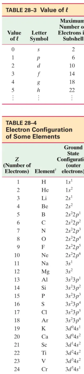
The Pauli exclusion principle limits the number of electrons possible in each shell and subshell. For any value of there are possible values ( can be any integer from 1 to from to or zero), and two possible values. There can be, therefore, at most electrons in any subshell. For
example, for five values are possible and for each
of these, can be or for a total of states. Table 28–3 lists the maximum number of electrons that can occupy each subshell.
Because the energy levels depend almost entirely on the values of nand it is customary to specify the electron configuration simply by giving the nvalue and the appropriate letter for with the number of electrons in each subshell given as a superscript. The ground-state configuration of sodium, for example, is written as
This is simplified in the Periodic Table by specifying the configuration only of the outermost electrons and any other nonfilled subshells (see Table 28–4 here, and the Periodic Table inside the back cover).
Electron configurations. Which of the following electron configurations are possible, and which are not: (a)
(b) (c)
RESPONSE (a) This is not allowed, because too many electrons (three) are
shown in the ssubshell of the M shell. The ssubshell has with two slots only, for “spin up” and “spin down” electrons.
(b) This is allowed, but it is an excited state. One of the electrons from the 3psubshell has jumped up to the 4ssubshell. Since there are 19 electrons, the element is potassium.
(c) This is not allowed, because there is no d subshell in the shell (Table 28–1). The outermost electron will have to be (at least) in the shell.
CONCEPTUAL EXAMPLE 28;6
1s22s22p63s1.
TABLE 28–3 Value of
Maximum Number of Value Letter Electrons in
of Symbol Subshell Electrons) Element† electrons)
1 H
†Names of elements can be found in
EXERCISE F Write the complete ground-state configuration for gallium, with its 31 electrons.
The grouping of atoms in the Periodic Table is according to increasing atomic number,Z. It was designed to also show regularity according to chemical prop-erties. Although this is treated in chemistry textbooks, we discuss it here briefly because it is a result of quantum mechanics. See the Periodic Table inside the back cover.
All the noble gases(in column VIII of the Periodic Table) have completely filled shells or subshells. That is, their outermost subshell is completely full, and the electron distribution is spherically symmetric. With such full spherical sym-metry, other electrons are not attracted nor are electrons readily lost (ionization energy is high). This is why the noble gases are chemically inert (more on this when we discuss molecules and bonding in Chapter 29). Column VII contains the halogens, which lack one electron from a filled shell. Because of the shapes of the orbits (see Section 29–1), an additional electron can be accepted from another atom, and hence these elements are quite reactive. They have a valence of meaning that when an extra electron is acquired, the resulting ion has a net charge of Column I of the Periodic Table contains the alkali metals, all of which have a single outer selectron. This electron spends most of its time outside the inner closed shells and subshells which shield it from most of the nuclear charge. Indeed, it is relatively far from the nucleus and is attracted to it by a net charge of only about because of the shielding effect of the other electrons. Hence this outer electron is easily removed and can spend much of its time around another atom, forming a molecule. This is why the alkali metals are very chemically reactive and have a valence of The other columns of the Periodic Table can be treated similarly.
The presence of the transition elementsin the center of the Periodic Table, as well as the lanthanides (rare earths) and actinides below, is a result of incomplete inner shells. For the lowest Zelements, the subshells are filled in a simple order: first 1s, then 2s, followed by 2p, 3s, and 3p.You might expect that 3d
would be filled next, but it isn’t. Instead, the 4slevel actually has a slightly lower energy than the 3d(due to electrons interacting with each other), so it fills first (K and Ca). Only then does the 3dshell start to fill up, beginning with Sc, as can be seen in Table 28–4. (The 4sand 3d levels are close, so some elements have only one 4selectron, such as Cr.) Most of the chemical properties of these transi-tion elements are governed by the relatively loosely held 4selectrons, and hence they usually have valences of or A similar effect is responsible for the lanthanidesandactinides, which are shown at the bottom of the Periodic Table for convenience. All have very similar chemical properties, which are determined by their two outer 6sor 7selectrons, whereas the different numbers of electrons in the unfilled inner shells have little effect.
28–9
X-Ray Spectra and
Atomic Number
The line spectra of atoms in the visible, UV, and IR regions of the EM spectrum are mainly due to transitions between states of the outer electrons. Much of the positive charge of the nucleus is shielded from these electrons by the negative charge on the inner electrons. But the innermost electrons in the shell “see” the full charge of the nucleus. Since the energy of a level is proportional to (see Eq. 27–15), for an atom with we would expect wavelengths about
times shorter than those found in the Lyman series of hydrogen
(around 100 nm), or to Such short wavelengths
lie in the X-ray region of the spectrum.
10–1nm. (100nm)兾(2500) L 10–2
502 = 2500
Z = 50,
Z2 n = 1
*
±2. ±1
(n =3,l=2)
±1. ±1e,
–1e. –1,
*SECTION 28–9 X-Ray Spectra and Atomic Number
817
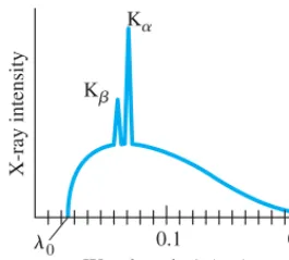
C A U T I O NX-rays are produced when electrons accelerated by a high voltage strike the metal target inside an X-ray tube (Section 25–11). If we look at the spectrum of wavelengths emitted by an X-ray tube, we see that the spectrum consists of two parts: a continuous spectrum with a cutoff at some which depends only on the voltage across the tube, and a series of peaks superimposed. A typical example is shown in Fig. 28–11. The smooth curve and the cutoff wavelength move to the left as the voltage across the tube increases. The sharp lines or peaks (labeled and in Fig. 28–11), however, remain at the same wavelength when the voltage is changed, although they are located at different wavelengths when different tar-get materials are used. This observation suggests that the peaks are characteristic of the target material used. Indeed, we can explain the peaks by imagining that the electrons accelerated by the high voltage of the tube can reach sufficient energies that, when they collide with the atoms of the target, they can knock out one of the very tightly held inner electrons. Then we explain these characteristic X-rays (the peaks in Fig. 28–11) as photons emitted when an electron in an upper state drops down to fill the vacated lower state. The K lines result from transitions into the K shell The line consists of photons emitted in a transition that originates from the (L) shell and drops to the (K) shell. On the other hand, the line reflects a transition from the (M) shell down to the K shell. An L line is due to a transition into the L shell, and so on.
Measurement of the characteristic X-ray spectra has allowed a determina-tion of the inner energy levels of atoms. It has also allowed the determinadetermina-tion of Zvalues for many atoms, because (as we have seen) the wavelength of the shortest characteristic X-rays emitted will be inversely proportional to Actually, for an electron jumping from, say, the to the level ( line), the wavelength is inversely proportional to because the nucleus is shielded by the one electron that still remains in the 1slevel. In 1914, H. G. J. Moseley (1887–1915) found that a plot of vs.Zproduced a straight line, Fig. 28–12, where is the wavelength of the line. The Zvalues of a number of elements were determined by fitting them to such a Moseley plot. The work of Moseley put the concept of atomic number on a firm experimental basis.
Ka
l
11兾l
(Z - 1)2
Ka n = 1
n = 2
Z2. n = 3
Kb
n = 1
n = 2
Ka (n = 1).
Kb
Ka
l0 l0
FIGURE 28–11 Spectrum of X-rays emitted from a molybdenum target in an X-ray tube operated at 50 kV.
Ka
0
X-ray intensity
Kb
Wavelength, l(nm) 0.2 0.1
l
FIGURE 28–12 Plot of vs.Z for X-ray Ka lines.
21兾l
Z 1
l
X-ray wavelength. Estimate the wavelength for an
to transition in molybdenum What is the energy of such a
photon?
APPROACH We use the Bohr formula, Eq. 27–16 for with replaced by
SOLUTION Equation 27–16 gives
where , , and . We substitute in values:
So
This is close to the measured value (Fig. 28–11) of 0.071 nm. Each of these photons would have energy (in eV) of:
The denominator includes the conversion factor from joules to eV. E = hf =
hc
l =
A6.63 * 10–34J
⭈sBA3.00 * 108m兾sB
A7.2 * 10–11mBA1.60 * 10–19J兾eVB = 17keV.
l =
1
1.38 * 1010m–1 = 0.072nm. 1
l = A1.097 * 10
7m–1B(41)2a1 1
-1
4b = 1.38 * 10 10m–1. k = 8.99 * 109
N⭈m2兾c2 n¿ = 1
n = 2
1
l = ¢
2p2e4 mk2
h3c ≤(Z - 1) 2¢ 1
n¿2 -1 n2≤ (Z - 1)2 = (41)2.
Z2 1兾l,
(Z = 42).
n = 1
Determining atomic number. High-energy electrons are used to bombard an unknown material. The strongest peak is found for X-rays emitted with an energy of 66.3 keV. Guess what the material is.
APPROACH The highest intensity X-rays are generally for the line (see
Fig. 28–11) which occurs when high-energy electrons knock out K shell elec-trons (the innermost orbit, ) and their place is taken by electrons from the L shell We use the Bohr model, and assume the electrons of the unknown atoms (Z) “see” a nuclear charge of (screened by one electron).
SOLUTION The hydrogen transition to would yield
(see Fig. 27–29 or Example 27–13). Energy of our unknown is proportional to (Eq. 27–15), or rather
because the nucleus is shielded by the one electron in a 1sstate (see above), so we can use ratios:
so and which makes it lead.
Now we briefly analyze the continuous part of an X-ray spectrum (Fig. 28–11) based on the photon theory of light. When electrons strike the target, they collide with atoms of the material and give up most of their energy as heat (about 99%, so X-ray tubes must be cooled). Electrons can also give up
energy by emitting a photon of light: an electron decelerated by interaction with atoms of the target (Fig. 28–13) emits radiation because of its deceleration (Chapter 22), and in this case it is called bremsstrahlung(German for “braking radiation”). Because energy is conserved, the energy of the emitted photon,hf,
equals the loss of kinetic energy of the electron, so
An electron may lose all or a part of its energy in such a collision. The continuous X-ray spectrum (Fig. 28–11) is explained as being due to such bremsstrahlung collisions in which varying amounts of energy are lost by the electrons. The shortest-wavelength X-ray (the highest frequency) must be due to an electron that gives up allits kinetic energy to produce one photon in a single collision. Since the initial kinetic energy of an electron is equal to the energy given it by the accelerating voltage,V, then In a single collision in which the electron
is brought to rest then and
We set where is the cutoff wavelength (Fig. 28–11) and find
(28;4)
This prediction for corresponds precisely with that observed experimentally. This result is further evidence that X-rays are a form of electromagnetic radiation (light) and that the photon theory of light is valid.
Cutoff wavelength. What is the shortest-wavelength X-ray photon emitted in an X-ray tube subjected to 50 kV?
APPROACH The electrons striking the target will have a ke of 50 keV. The
shortest-wavelength photons are due to collisions in which all of the electron’s
KEis given to the photon so
SOLUTION From Eq. 28–4,
or 0.025 nm.
NOTE This result agrees well with experiment, Fig. 28–11.
l0 =
hc eV =
A6.63 * 10–34J
⭈sBA3.0 * 108m兾sB
A1.6 * 10–19CBA5.0 * 104VB = 2.5 * 10
–11 m,
ke = eV = hf0.
EXAMPLE 28;9 l0
l0 =
hc eV.
l0 f0 = c兾l0
hf0 = eV.
¢ke = eV
(ke¿ = 0),
ke = eV.
hf = ¢ke.
¢ke = ke - ke¿,
Z = 82,
Z - 1 = 16500 = 81,
EZ
EH =
(Z - 1)2
12 =
66.3 * 103eV
10.2eV = 6.50 * 10 3
,
(Z - 1)2 Z2
EZ
EH = 13.6eV - 3.4eV = 10.2eV
n = 1
n = 2
Z - 1
(n = 2).
n = 1
Ka
EXAMPLE 28;8
*SECTION 28–9 X-Ray Spectra and Atomic Number
819
FIGURE 28–13 Bremsstrahlung photon produced by an electron decelerated by interaction with a target atom.
KE⬘ KE
Photon hf =KE−KE⬘
+ –
28–10
Fluorescence and Phosphorescence
When an atom is excited from one energy state to a higher one by the absorption of a photon, it may return to the lower level in a series of two (or more) transitions if there is at least one energy level in between (Fig. 28–14). The photons emitted will consequently have lower energy and frequency than the absorbed photon. When the absorbed photon is in the UV and the emitted photons are in the visible region of the spectrum, this phenomenon is called fluorescence (Fig. 28–15).The wavelength for which fluorescence will occur depends on the energy levels of the particular atoms. Because the frequencies are different for different sub-stances, and because many substances fluoresce readily, fluorescence is a powerful tool for identification of compounds. It is also used for assaying—determining how much of a substance is present—and for following substances along a natural metabolic pathwayin biological organisms. For detection of a given compound, the
stimulating light must be monochromatic, and solvents or other materials present must not fluoresce in the same region of the spectrum. Sometimes the observation of fluorescent light being emitted is sufficient to detect a compound. In other cases, spectrometers are used to measure the wavelengths and intensities of the emitted light.
Fluorescent lightbulbswork in a two-step process. The applied voltage accel-erates electrons that strike atoms of the gas in the tube and cause them to be excited. When the excited atoms jump down to their normal levels, they emit UV photons which strike a fluorescent coating on the inside of the tube. The light we see is a result of this material fluorescing in response to the UV light striking it.
Materials such as those used for luminous watch dials, and other glow-in-the-dark products, are said to be phosphorescent. When an atom is raised to a normal excited state, it drops back down within about In phosphorescent substances, atoms can be excited by photon absorption to energy levels called metastable, which are states that last much longer because to jump down is a “forbidden” transition (Section 28–6). Metastable states can last even a few seconds or longer. In a collection of such atoms, many of the atoms will descend to the lower state fairly soon, but many will remain in the excited state for over an hour. Hence light will be emitted even after long periods. When you put a luminous watch dial close to a bright lamp, many atoms are excited to metastable states, and you can see the glow for a long time afterward.
28–11
Lasers
Alaseris a device that can produce a very narrow intense beam of monochromatic coherent light. (By coherent, we mean that across any cross section of the beam, all parts have the same phase.†) The emitted beam is a nearly perfect plane wave.
An ordinary light source, on the other hand, emits light in all directions (so the intensity decreases rapidly with distance), and the emitted light is incoherent (the different parts of the beam are not in phase with each other). The excited atoms that emit the light in an ordinary lightbulb act independently, so each photon emitted can be considered as a short wave train lasting about Different wave trains bear no phase relation to one another. Just the opposite is true of lasers.
The action of a laser is based on quantum theory. We have seen that a photon can be absorbed by an atom if (and only if) the photon energy hfcorresponds to the energy difference between an occupied energy level of the atom and an avail-able excited state, Fig. 28–16a. If the atom is already in the excited state, it may jump down spontaneously (i.e., no stimulus) to the lower state with the emission of a photon. However, if a photon with this same energy strikes the excited atom, it can stimulate the atom to make the transition sooner to the lower state, Fig. 28–16b. This phenomenon is called stimulated emission: not only do we still have the original photon, but also a second one of the same frequency as a result
10–8s. 10–8s.
*
P H Y S I C S A P P L I E D
Fluorescence analysis and fluorescent lightbulbs
FIGURE 28–14 Fluorescence.
FIGURE 28–15 When UV light (a range of wavelengths) illuminates these various “fluorescent” rocks, they fluoresce in the visible region of the spectrum.
FIGURE 28–16 (a) Absorption of a photon. (b) Stimulated emission.
and refer to “upper” and “lower” energy states.
El Eu
One photon absorbed
Two photons emitted
(a) hf =E
u−El
hf =Eu−El Eu hf
El
(b)
Eu hf
of the atom’s transition. These two photons are exactly in phase, and they are moving in the same direction. This is how coherent light is produced in a laser. The name “laser” is an acronym for LightAmplification by StimulatedEmission ofRadiation.
Normally, most atoms are in the lower state, so the majority of incident pho-tons will be absorbed. To obtain the coherent light from stimulated emission, two conditions must be satisfied. First, the atoms must be excited to the higher state so that an inverted populationis produced in which more atoms are in the upper state than in the lower one (Fig. 28–17). Then emissionof photons will dominate over absorption. And second, the higher state must be a metastable state—a state in which the electrons remain longer than usual†so that the transition to the lower
state occurs by stimulated emission rather than spontaneously.
Figure 28–18 is a schematic diagram of a laser: the “lasing” material is placed in a long narrow tube at the ends of which are two mirrors, one of which is partially transparent (transmitting perhaps 1 or 2%). Some of the excited atoms drop
down fairly soon after being excited. One of these is the blue atom shown on the far left in Fig. 28–18. If the emitted photon strikes another atom in the excited state, it stimulates this atom to emit a photon of the samefrequency, moving in the same direction, and in phasewith it. These two photons then move on to strike other atoms causing more stimulated emission. As the process continues, the number of photons multiplies. When the photons strike the end mirrors, most are reflected back, and as they move in the opposite direction, they continue to stimulate more atoms to emit photons. As the photons move back and forth between the mirrors, a small percentage passes through the partially transparent mirror at one end. These photons make up the narrow coherent external laser beam. (Inside the tube, some spontaneously emitted photons will be emitted at an angle to the axis, and these will merely go out the side of the tube and not affect the narrow width of the main beam.)
SECTION 28–11 Lasers
821
†An excited atom may land in such a state and can jump to a lower state only by a so-called forbiddentransition (Section 28–6), which is why its lifetime is longer than normal.
FIGURE 28–17 Two energy levels for a collection of atoms. Each dot represents the energy state of one atom. (a) A normal situation; (b) an inverted population.
Normal population
(a)
Inverted population
(b)
FIGURE 28–18 Laser diagram, showing excited atoms stimulated to emit light. Mirror
Partially transparent mirror
Laser output beam
In a well-designed laser, the spreading of the beam is limited only by diffrac-tion, so the angular spread is (see Eq. 24–3 or 25–7) where Dis the diameter of the end mirror. The diffraction spreading can be incredibly small. The light energy, instead of spreading out in space as it does for an ordinary light source, can be a pencil-thin beam.
Creating an Inverted Population
The excitation of the atoms in a laser can be done in several ways to produce the necessary inverted population. In a ruby laser, the lasing material is a ruby rod consisting of with a small percentage of aluminum (Al) atoms replaced by chromium (Cr) atoms. The Cr atoms are the ones involved in lasing. In a process calledoptical pumping, the atoms are excited by strong flashes of light of wave-length 550 nm, which corresponds to a photon energy of 2.2 eV. As shown in Fig. 28–19, the atoms are excited from state to state The atoms quickly decay either back to or to the intermediate state which is metastable with a lifetime of about (compared to for ordinary levels). With strong pumping action, more atoms can be found in the state than are in the state. Thus we have the inverted population needed for lasing. As soon as a few atoms in the state jump down to they emit photons that produce stimulated emission of the other atoms, and the lasing action begins. A ruby laser thus emits a beam whose photons have energy 1.8 eV and a wavelength of 694.3 nm (or “ruby-red” light).
E0, E1
E0 E1
10–8s 3 * 10–3s
E1, E0
E2. E0
Al2O3
Ll兾D
FIGURE 28–19 Energy levels of chromium in a ruby crystal. Photons of energy 2.2 eV “pump” atoms from
to which then decay to metastable state Lasing action occurs by stimulated emission of photons in transition from E1to E0.
E1. E2,
E0
2.2 eV 1.8 eV 0.4 eV
E2
E1
E0
(metastable) C A U T I O N
Laser: photons have

![FIGURE 28–9 Electron cloud, orprobability distribution, for states in hydrogen. [The donut-shaped orbit in (c) is the sum of twodumbbell-shaped orbits, as in (b),along the x and y axes addedtogether.]n = 2](https://thumb-ap.123doks.com/thumbv2/123dok/2189445.1618157/13.613.41.173.81.524/figure-electron-orprobability-distribution-states-hydrogen-twodumbbell-addedtogether.webp)