© Author(s) 2017. CC BY-NC-ND Attribution 4.0 License.
Temporal decorrelation effect in carbon stocks estimation using
Polarimetric Interferometry Synthetic Aperture Radar (PolInSAR)
(case study: Southeast Sulawesi tropical forest)
Laode Muh. Golok Jaya*,1,2, Ketut Wikantika2,3, Katmoko Ari Sambodo4, Armi Susandi5 1 Faculty of Engineering, Universitas Halu Oleo, Jl. HEA. Mokodompit No. 8, Kampus Hijau UHO, Anduonohu Kendari
Southeast Sulawesi (Indonesia)
2 Center for Remote Sensing Institute of Technology Bandung (ITB) Jl. Ganesha No. 10, Bandung, West Java (Indonesia), 3 ForMIND Institute (Forum Peneliti Muda Indonesia)
4 Indonesia National Institute of Aeronautics and Space (LAPAN) Jl. Lapan No. 70, Pekayon Pasar Rebo, Jakarta
(Indonesia)
5 Meteorology Department, Faculty of Earth Science and Technology, ITB (Indonesia), Jl. Ganesha No. 10, Bandung West
Java (Indonesia)
* Corresponding Author (e-mail: [email protected])
Received: 30 March 2017 / Accepted: 13 April 2017 / Published: 01 July 2017
Abstract.This paper was aimed to analyse the effect of temporal decorrelation in carbon stocks estimation. Estimation of carbon stocks plays important roles particularly to understand the global carbon cycle in the atmosphere regarding with climate change mitigation effort. PolInSAR technique combines the advantages of Polarimetric Synthetic Aperture Radar (PolSAR) and Interferometry Synthetic Aperture Radar (InSAR) technique, which is evidenced to have significant contribution in radar mapping technology in the last few years. In carbon stocks estimation, PolInSAR provides information about vertical vegetation structure to estimate carbon stocks in the forest layers. Two coherence Synthetic Aperture Radar (SAR) images of ALOS PALSAR full-polarimetric with 46 days temporal baseline were used in this research. The study was carried out in Southeast Sulawesi tropical forest. The research method was by comparing three interferometric phase coherence images affected by temporal decorrelation and their impacts on Random Volume over Ground (RvoG) model. This research showed that 46 days temporal baseline has a significant impact to estimate tree heights of the forest cover where the accuracy decrease from R2=0.7525 (standard deviation of tree heights is 2.75 meters) to R2=0.4435 (standard deviation 4.68 meters) and R2=0.3772 (standard deviation 3.15 meters) respectively. However, coherence optimisation can provide the best coherence image to produce a good accuracy of carbon stocks.
Keywords:Temporal Decorrelation, Carbon Stocks, PolInSAR, ALOS PALSAR.
Abstrak. Penelitian ini bertujuan untuk meneliti pengaruh dekorelasi temporal dalam
pendugaan cadangan karbon. Pendugaan cadangan karbon sangat penting untuk memahami daur karbon secara global in atmosfer terkait upaya mitigasi perubahan iklim. Teknik PolInSAR menggabungkan dua buah teknik pemetaan dengan citra Synthetic Aperture Radar (SAR) yaitu Polarimetric Synthetic Aperture Radar (PolSAR) dan Interferometry Synthetic Aperture Radar (InSAR) yang terbukti berkontribusi dalam teknologi pemetaan sejak beberapa tahun terakhir. Teknik PolInSAR dapat memberikan informasi struktur tinggi vegetasi yang digunakan untuk menduga besarnya cadangan karbon pada tutupan hutan. Dua buah citra ALOS PALSAR yang koheren dan full-polarisasi dengan perbedaan waktu perekaman 46 hari digunakan dalam penelitian ini. Wilayah studi penelitian ini adalah hutan tropis Sulawesi Tenggara. Metode penelitian ini adalah membandingkan tiga buah citra fase interferometrik yang dipengaruhi oleh dekorelasi temporal dan dampaknya dalam pembentukan model RVoG. Hasil penelitian ini menunjukkan bahwa adanya perbedaan perekaman citra selama
46 hari memiliki dampak yang signifikan dalam estimasi cadangan karbon dimana akurasi
(simpangan baku 4.68 meter) dan R2=0.3772 (simpangan baku 3.15 meter). Namun demikian,
dengan proses optimisasi koherensi dapat menghasilkan citra dengan nilai koherensi yang terbaik untuk menghasilkan nilai cadangan karbon dengan akurasi yang baik.
Kata Kunci:Dekorelasi Temporal, Cadangan Karbon, PolInSAR, ALOS PALSAR
1. Introduction
Estimation of carbon stocks plays an important role in the context of climate change mitigation. Forest layers absorb carbon emission from the atmosphere and store it as carbon pool (IPCC, 2007). Indonesia is one of the countries having the largest tropical forest that contains carbon stocks and gives impact to climate change. The mapping of forest carbon stocks in Indonesia will be very useful to support mitigation of climate change under the scheme of Reducing Emission from Deforestation and Forest Degradation (REDD). Some efforts have been conducted to estimate carbon stocks of Indonesian tropical forest including by using optical remote sensing (Kustiyo et al, 2015). However, optical remote sensing system does not generate optimum results such as the unclear and low quality of satellite image due to cloud cover and other meteorological conditions. Therefore, the radar remote sensing system becomes another option and has been widely applied for that purpose. In the model development for carbon stocks mapping, radar polarimetric (PolSAR) has been popular in the last few years. Radar polarimetric uses polarisation component to develop the relationship between forest
carbon stocks and backscatter coefficient from
different frequencies (Mitchell et al, 2012; Villard & Le Toan, 2014) and different sensors (Kurvonen et al, 1999). However, this method has a problem of saturation (Moreira et al, 2002; Le Toan et al, 2011). Meanwhile, radar interferometric (InSAR) has some advantages
including it is not influenced by saturation.
Some researchers such as Neeff et al, (2005) and Kugler et al, (2006) have discussed the contribution of the InSAR method to assess
biophysical parameters in forest areas. Thus, the integration of radar polarimetry and interferometry (PolInSAR) can overcome saturation problem in the development of physical object model. This method was initially published by Cloude and Papathanassiou (1998). The PolInSAR is based on the formation of two coherence images from two difference positions and times of acquisition. It means that the PolInSAR is particularly vulnerable to temporal decorrelation (Mette, 2006; Richards, 2009). The objective of this paper was to analyse the effects of temporal decorrelation in carbon stocks estimation using ALOS PALSAR full-polarimetric image.
2. Research Method a. Location
This research was conducted in Southeast
Sulawesi, Indonesia. Specifically, the study are
is a part of Wolasi Tropical Protection Forest (4°06’10.22”S to 4°12’15.74”S and 122°29’2.15”E to 122°30’33.4”E) and the altitude at 300-700 meter above mean sea level. The average temperature is 25 –34° and annual precipitation is 1,469 mm. The topography is mountainous with a gradient up to 10-20%. Furthermore, 20 sample plots were established in the study area with 20x20m2 in size. The map of the study area is displayed in Figure 1.
The dominant vegetations in this area are
Eha (Castanopsis buruana), Batu-Batu (Ptemandra spp.), Dange (Dillenia sp.) and Ruruhi (Syzygium spp.). Some of trees aged between 5 (five) to
Figure 1. Map of study area based on SRTM data of Southeast Sulawesi, Indonesia. White rectangle indicates position of ALOS PALSAR data coverage used in this study.
Figure 2. (a) Situation of forest in the study area, (b) one of dominant tree species: Eha (Castanopsis buruana).
b. SAR Data
Two levels of L1.1 full polarimetric ALOS PALSAR data were used in this research. The polarisations were HH, HV, VH and VV,
respectively. Temporal baseline between these two images was 46 days. Data characteristics are described in Table 1. The images were divided into master and slave.
Table 1. ALOS PALSAR data characteristics
Description Master Image Slave Image
Center Frequency 1,25 GHz 1,25 GHz
Wavelength 23 cm 23 cm
Polarization HH, HV, VH, VV HH, HV, VH, VV
Range Resolution 9.4 m 9.4 m
Azimuth Resolution 3.8 m 3.6 m
Date of acquisition 2 May 2010 17 March 2010
Incidence Angle 23° 21.5°
Pass Ascending Ascending
c. SAR Data Processing
SAR data processing is a fundamental key to obtain good quality of interferogram. Its fundamental steps consist of multilooking, polarimetric calibration,
coregistration, spectral filtering and
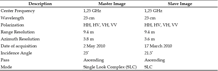
interferogram generation. It also proceeds two coherence ALOS PALSAR images from two different periods and two slightly different look angles, further referred as master and slave as presented in Figure 3 in Red Green Blue (RGB) composite.
Figure 3. Pairs of ALOS PALSAR images in RGB composite (HH, HV, HH/HV): (a) image assigned as master and (b) slave.
PolInSAR technique is an integration of the advantages of PolSAR and InSAR techniques. The coherence between two identical images in full-polarizations environment is the key of PolInSAR technique (Cloude & Papathanossiou, 1998). ALOS PALSAR image obtained on May 2nd, 2010 was assigned as master image and those on March 17th, 2010 was assigned as slave. Each image was performed as scattering matrix contains all polarisations as displayed in equation (1).
(1)
The scattering matrix, namely the S2 matrix, contains backscatter properties of the earth objects (Richards, 2009). The scattering matrix characterises the scattered wave for any polarisation of incidence wave at every image pixel. The elements of the scattering matrix are very useful in the analysis of pixels, for
example, on the classification process using
decomposition (Richards, 2009). The matrix component can be transformed into a vector with four elements arranged in the form of the scattering matrix-vector, called Pauli basis target vector (Cloude & Papathanossiou, 1998; Richards, 2009) as shown in Equation (2). “T” indicates transpose matrix.
(2)
For coregistration of two full polarimetric SAR coherent images, equation (2), was
(3)
Where < > represented multi-looking operator, * is Hermitian transformation, k1 and k2 are 3D Pauli scattering vectors. and are standard Hermitian coherency matrix containing polarimetric information from each full-polarimetric image. The matrix states new complex matrix in 3x3 dimension, which contains not only polarimetric information, but also interferometric phase between polarimetric channels in the coherent pair images (Richards, 2009). The T6 was then proceeded to estimate the coherence of interferogram and to produce the RVoG model.
3. Results and Discussion
Estimation of carbon stocks in Indonesia has been carried out by several researchers by using several ways, including backscatter radar to identify the characteristics of forest stand in tropical forest (Wuryanta, 2016), discrimination of mangrove ecosystem objects on the visible spectrum using spectroradiometer HR-1024 (Arfan, 2015) and calculation based on land cover changes in the Leuser Ecosystem Area (LEA) in Aceh (Hermon, 2015). However, the efforts produced uncertainty results. In this paper, we attempted to minimise the uncertainty by using PolInSAR method and to investigate the impediment aspect, namely the temporal decorrelation.
In Indonesia, the usage of PolInSAR through INDREX-II airborne campaign was initiated in 2004 (Hajnsek et al, 2005). The campaign was conducted to develop database of aboveground biomass in Kalimantan forests by using L- and P-bands in polarimetric and interferometric components using Experimental Synthetic Aperture Radar (E-SAR) of the German Aerospace Center (DLR). Radar technology is allegedly suitable to map carbon stocks in Indonesian forest environment due to the obstacles of cloud cover, smoke and haze, especially in Sumatera, Kalimantan, Sulawesi and Papua.
Temporal Decorrelation is the main problem in the PolInSAR (Mette, 2006; Richards,
2009; Meng et al, 2010). Decorrelation itself is divided into two ways. First, it refers to the critical baseline. A larger baseline means a greater phase shift leads to a more sensitive interferometer. However, there is a limit at
2π phase shift for certain pixels. If the change exceeds 2π , then it is hard to recover the
inter-pixel variation in elevation (Richard, 2009). He also suggested that the > 1000m baseline of
spaceborne will inhibit to understand the flat
earth variation. In relation with airborne SAR image, Lee and Pottier (2009) explained their preference to use 10 m baseline pair in their study in order to avoid phase unwrapping problems in forest height estimation as well as 20 m baseline to gain better sensitivity in height estimation, which could be used for height estimation of lower vegetation. Second, decorrelation comes from any mechanism that leads to statistical differences between the signals received by two channels (Richards, 2009). Repeat-pass interferometry will change ground scattered in two acquisitions then the interferometric phase difference will be affected. Shortly, temporal decorrelation will lead to uncertainty in interferogram formation. However, it cannot be avoided in repeat-pass mode of SAR system, for instance ALOS PALSAR. To reduce the impact of temporal decorrelation, coherence optimisation was conducted.
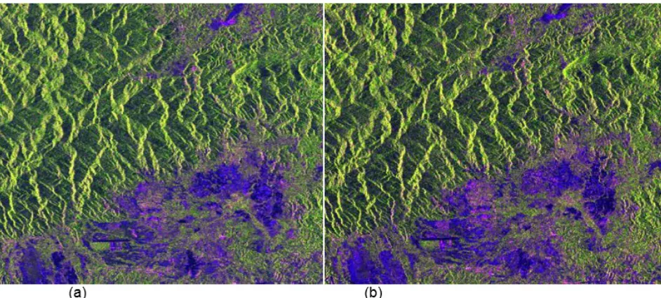
Figure 4, 5, and 6 showed the coherence level between pair of images produced by coherence optimisation. Coherence value will be zero (0) for minimum called incoherence (black colour) and one (1) for maximum called fully coherence (white colour). Indicated by the histogram of coherence, Figure 4 is identified as the best coherence since the histogram value is near to one. The optimum coherence value was obtained by ground topography but dropped down in the forested area because of the residual volume component which cannot be removed (Cloude & Papathanassiou, 2003).
establish Random Volume over Ground (RVoG) model. RVoG is biophysical model of forest which is separated into two layers; top canopy layer and underlying topography (Cloude & Papathanassiou, 2003). Figure 4 showed the
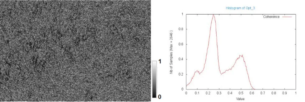
most coherent image in compared to Figure 5 and 6, in which Figure 5 is more coherent than 6. The effect of temporal decorrelation can be observed in forest height inversion from RVoG model as showed in Figure 7 (a), (b) and (c).
Figure 4. Optimised interferometric coherence #1 (OPT_1) and its histogram.
Figure 5. Optimised interferometric coherence #2 (OPT_2) and its histogram.
Figure 7. Forest height from RVoG model. (a) from optimized interferometric coherence #1 (OPT_1), (b) optimized interferometric coherence #2 (OPT_2), and (c) optimized interferometric coherence #3 (OPT_3).
Figure 8. Temporal decorrelation effect on the accuracy of forest heights (a) from optimized interferometric coherence #1 (OPT_1), (b) optimized interferometric coherence #2 (OPT_2), and (c) optimized interferometric coherence #3
(OPT_3).
Temporal decorrelation affected not only the inaccuracy of forest heights but also the decline of the top phase height of forest canopy layer. In this research, the maximum canopy layer height decreased by 22%, from 32 m to 25 m as an effect of temporal decorrelation. Furthermore, the accuracy of forest height obtained from field survey In compared to RVoG heights also decreased.
Figure 8 (a), (b) and (c) showed the effect of temporal decorrelation on the accuracy of canopy layer heights. The accuracy decreased from R2=0.7525 (standard deviation of tree heights is 2.75 meters) to R2=0.4435 (standard deviation 4.68 meters) and R2=0.3772 (standard deviation 3.15 meters), respectively. In the repeat-pass mode, the temporal decorrelation cannot be avoided (Askne & Santoro, 2005; Lee etal., 2009). Hence, spaceborne single pass mode program, e.g., TanDEM-X has been developed to overcome the temporal decorrelation (Kugler etal., 2014). However, from this research, it can be suggested to consider the effect of temporal decorrelation in PolInSAR technique to minimise the uncertainty of carbon estimation in the context of climate change mitigation. Consequently, coherence optimisation must be
conducted to get the highest accuracy of tree heights estimation (Lee & Pottier, 2009). Thus the highest accuracy carbon stocks can be gained.
4. Conclusions
5. Acknowledgment
We would like to thank Prof. M Shimada from JAXA Japan who provided ALOS PALSAR Full-Polarimetric. Also thanks to our
colleagues at Faculty of Forestry and Faculty of Engineering Universitas Halu Oleo, CRS ITB, and ForMIND Institute (Prof. Ketut Wikantika) for the assistances in completing this work.
6. References
Arfan, A. (2015) Discrimination of Mangrove Ecosystem Objects on the Visible Spectrum Using Spectroradiometer HR-1024, Forum Geografi, Vol. 29 (1), pp.83 – 88.
Askne, J. and Santoro, M. (2005) Multitemporal repeat-pass SAR interferometry of boreal forest, IEEE Transactions on Geoscience and Remote Sensing, 43: 1219-1228.
Cloude, S.R and Papathanassiou, K. (1998) Polarimetric SAR Interferometry, IEEE Transactions on Geoscience and Remote Sensing, Vol. 36 No. 5, pp. 1551-1565.
Cloude, S.R and Papathanassiou, K. (2003) Three-stage inversion process for Polarimetric SAR Interferometry, IEE Proc-Radar Sonar Navigation, 150: 125-134.
Florian, K., Papathanassiou K., Hajnsek, I. and Dirk, H. (2006) Forest height estimation in tropical rain forest using Pol-Insar techniques, German Aerospace Center (DLR), IEEE 0-7803-9510-7/06.
Hajnsek, I., Kugler, F., Papathanossiou, K., Horn, R., Schieber, R., Moreira, A., Hoekman, D., Davidson, M. (2005) INDREX II – Indonesian airborne radar experiment campaign over tropical forest in L- and P- band: first results, Proceedings of Geoscience and Remote Sensing Symposium 2005 (IGRASS 2005) Page(s): 4335-4338, July 25-29, 2005, Seoul, South Korea. Hermon, D. (2015) Estimate of Changes in Carbon Stocks Based on Land Cover Changes in the
Leuser Ecosystem Area (LEA) Indonesia, Forum Geografi, Vol 29 (2), pp. 187-196.
IPCC (Inter-Governmental Panel on Climate Change) (2007) The Carbon Cycle and Atmospheric Carbon Dioxide Content.
Kugler, F., Papathanassiou K.P., Hajnsek I. (2006) Forest height estimation over tropical forest by means of polarimetric SAR interferometry. Proceedings of: VII Seminário de Atualização em Sensoriamento Remoto e Sistemas de Informações Geográficas Aplicados à Engenharia Florestal, October 2006. Curitiba: 504–512.
Kugler, F., Schulze, D., Hajnsek, I., Pretzsch, H. and Papathanassiou, K.P. (2014) TanDEM-X Pol-InSAR Performance for Forest Height Estimation, IEEE Transactions on Geoscience and Remote Sensing, DOI:10.1109/TGRS. 2013.2296533.
Kurvonen, L., Pulliainen, J., and Hallikainen, M. (1999) Retrieval of biomass in boreal forest from multitemporal ERS-1 and JERS-1 SAR images, IEEE Transactions on Geoscience and Remote Sensing, 37, pp. 198-205.
Kustiyo, O. Roswintiarti, A. Tjahjaningsih, R. Dewanti, S. Furby, J. W. (2015) Annual Forest Monitoring as Part of the Indonesia’s National Carbon Accounting System, The International Archives of the Photogrammetry, Remote Sensing and Spatial Information Sciences, Volume XL-7/W3, 36th International Symposium on Remote Sensing of Environment, Berlin, Germany.
Lee, S.K., Kugler, F., Papathanassiou, K.P., and Moreira, A. (2009) Forest Height Estimation by means of Pol-InSAR Limitations posed by Temporal Decorrelation, K&C Science Report – Phase 1, Microwaves and Radar Institute (DLR-HR), German Aerospace Center (DLR). Lee, J. and Pottier, E. (2009) Polarimetric Radar Imaging from Basics to Applications, CRC Press,
ISBN 978-1-4200-5497-2.
global forest biomass to better understand the terrestrial carbon cycle, Remote sensing of Environment 115, pp. 2850-2860.
Meng, W. and Sandwell DT. (2010) Decorrelation of L-band and C-band interferometry over vegetated areas in California, IEEE Transactions on Geoscience and Remote Sensing, 48: 2942-2952.
Mette, T., Papathanassiou, K.P., Hajnsek, I., Zimmermann, R. (2003) Forest Biomass Estimation using Polarimetric SAR Interferometry.
Mette, T. (2006) Forest Biomass Estimation from Polarimetric SAR Interferometry, Dissertation, Technischen Universität München.
Mitchell, A.L., Williams, M., Tapley, I., Milne, A.K. (2012) Interoperability of Multi-Frequency SAR Data for Forest Information Extraction in Support of National MRV System, IEEE Trans. on Geoscience and Remote Sensing.
Moreira, A., Papathanassiou, K., Krieger, G. (2002) Polarimetric SAR Interferometry with a Passive Polarimetric Micro-Satellite Concept, Institute of Radio Frequency Technology and Radar Systems, German Aerospace Center (DLR).
Neeff, T., Biging G.S., Dutra L.V., Freitas C.C. and Santos J.R. (2005) Modeling spatial tree pattern in the Tapajós forest using interferometric height, Revista Brasileira de Cartografia 57 (1): 1–6.
Richards, J. A. (2009) Remote Sensing with Imaging Radar, Signals and Communication Technology, ISBN: 978-3-642-02019-3, Springer.
Villard, L. and Le Toan, T. (2014) Relating P-Band SAR Intensity to Biomass for Tropical Dense Forests in Hilly Terrain: γ0 or t0?, IEEE Journal of Selected Topics in Applied Earth Observations and Remote Sensing.
© Author(s) 2017. CC BY-NC-ND Attribution 4.0 License.
Impacts of Extreme Weather on Sea Surface Temperature in the
Western Waters of Sumatera and the South of Java in June 2016
Martono
Centre of Atmospheric Science and Technology (LAPAN) Jl. Dr. Djundjunan 133 Bandung, West Java Corresponding author (e-mail: [email protected])
Received: 13 January 2017 / Accepted: 05 February 2017 / Published: 01 July 2017
Abstract.Ocean dynamics are affected by the condition of the weather. Surface wind is one of the weather elements that has an important role on the ocean dynamics. This research was conducted to determine the impacts of extreme weather on sea surface temperature in the western waters of Sumatra and the southern waters of Java in June 2016. Data analysed in this study consisted of daily surface wind from 2007 to 2016, daily sea surface temperature from 1987 to 2016, and surface current from 1994 to 2016. The method used in this research was anomaly analysis. The result showed that in June 2016, extreme weather occurred in those waters. The impacts of extreme weather in the western waters of Sumatra and the southern waters of Java caused lower upwelling intensity that was indicated by an increase of sea surface temperature. The Increases of sea surface temperature in the BS1, BS2, SJ were 0.9ºC, 1.8ºC, and 1.6ºC, respectively.
Keywords:Impacts, extreme weather, sea surface temperature, upwelling.
Abstrak.Dinamika laut dipengaruhi oleh kondisi cuaca. Angin permukaan merupakan salah
satu unsur cuaca yang mempunyai peranan penting terhadap dinamika laut. Penelitian ini dilakukan untuk mengetahui dampak cuaca ekstrim terhadap suhu permukaan laut di perairan barat Sumatera dan selatan Jawa. Data yang digunakan terdiri dari angin harian dari 2007-2016, suhu permukaan laut harian dari 1987-2016 dan arus permukaan dari 1994-2016. Metode yang digunakan dalam penelitian ini adalah analisis anomali. Hasil penelitian menunjukkan bahwa selama bulan Juni 2016 telah terjadi kondisi cuaca ekstrim di perairan ini. Dampak cuaca ekstrim di perairan barat Sumatera dan selatan Jawa menyebabkan intensitas upwelling melemah yang ditandai dengan kenaikan suhu permukaan laut. Kenaikan suhu permukaan laut di BS1 mencapai 0,9ºC, di BS2 1,8ºC dan di SJ mencapai 1,6ºC.
Kata Kunci:dampak, cuaca ekstrem, suhu permukaan laut, upwelling.
1. Introduction
The dynamics of the marine
environment are strongly influenced by
the weather condition, hence, any change of the weather will affect the dynamics of the marine environment. Surface wind is the main factor of dynamics of marine waters. Energy transfer from surface wind to sea surface will generate surface current and wave (Dahuri etal., 1996; Ibrayev etal., 2010). Surface wind is also one element of climate control (Tjasyono, 2004).
Ocean dynamics of the western waters of Sumatra and the southern waters of Java are unique and complex since the waters
are affected by the monsoon system (Shenoi
etal., 1999; Yoga etal., 2014). The monsoon system occurs due to the difference between the high air pressure and the low air pressure above the Asia and Australia continent. The monsoon system changes its direction once a year. One of the ocean events that occurs in the western waters of Sumatra and the southern waters of Java due to the monsoon system is upwelling events.
Upwelling events generally increase the waters productivity. Therefore, the locations where upwelling occurs have
high potential of fisheries. Research about
by several researchers among others Wyrtki
(1961), Susanto, et al., (2001), Kunarso, et al.,
(2005), Kunarso, et al., (2011), Susanto and
Marra (2005), Qu, et al., (2005), Kemili dan
Putri (2012), and Syafik, et al., (2013). The most
common method to determine upwelling events is by observing the data of sea surface temperature (Aldrian, 2008).
Extreme temperature and precipitation in
Indonesia have been identified by Supari et al., (2016a) and in Borneo by Supari et al., (2016b). However, the investigation of the extent of such events to affect the potential of sea surface rise is important since there is an interaction between air temperature and sea surface as well as between precipitation and sea level (Martono, 2016; Supriatin & Martono, 2016). In the beginning of June 2016, extreme weather occurred in the western waters of Sumatra and
the southern waters of Java. The purpose of this study was to determine the impacts of extreme weather on sea surface temperature and sea surface rise in the western waters of Sumatra and the southern waters of Java in June 2016.
2. Research Method
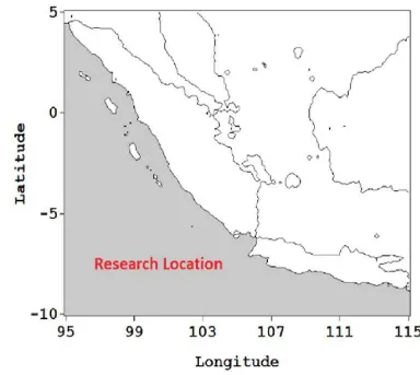
The study area was the western waters of Sumatra and the southern waters of Java situated at 6° N - 10° S and 95° E - 114° E as shown in Figure 1. For the analysis purposes, the study area was divided into three parts: 1). BS1 which was the western waters of Sumatra from the middle part of the waters to the northern part; 2). BS2 which was the western waters of Sumatra from the middle part to the southern part; and 3). SJ which was the southern waters of Java.
Figure 1. The study area.
The data collected for the analysis consisted of daily surface wind from 2007 to 2016, daily sea surface temperature from 1987 to 2016, daily
obtained from the Centre ERS d’Archivage et de Traitement - French Research Institute for Exploitation of the Sea; sea surface temperature data with 0.25° spatial resolution was obtained from the Physical Oceanography Distributed Active Archive Center NASA; sea level height anomaly data with 0.25° spatial resolution and
surface current data with 1° spatial resolution were obtained from the Ocean Surface Current Analysis Real-Time NOAA.
Method used in this research was anomaly analysis. The value of SST anomaly was calculated by the equation:
(1)
Where SSTA is the value of SST anomalies and is the climatological value of SST.
3. Results and Discussion
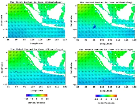
The climatological pattern of surface wind in the western waters of Sumatera and the
southern waters of Java from the first to the
fourth pentad in June 2016 is demonstrated in
Figure 2. Generally, there are two patterns of surface wind in the western waters of Sumatra
during the specific time. In BS1, the surface
wind blew to the northeast, meanwhile it blew to the north-west in BS2. The pattern of surface wind in SJ was the surface wind blew to the west.
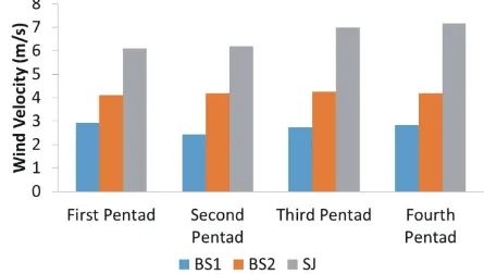
Figure 3 shows the mean velocity of
surface wind from the first to fourth pentad
in the western waters of Sumatra and the southern waters of Java in June 2016. The mean velocity of surface wind in BS1 was higher than those of BS2 and the highest value was obtained by SJ. The values of mean velocity of
surface wind of BS1, BS2, and SJ were 4.2 m/s, 2.7 m/s, and 6.6 m/s, respectively. Intensity
of surface wind velocity from the first until
the fourth pentad in the western waters of Sumatra was almost similar, meanwhile, there was an increased velocity in the southern waters of Java.
Figure 3. Climatological mean surface wind velocity in June 2016.
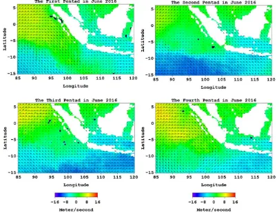
Patterns of surface wind over the western waters of Sumatra and the southern waters of Java in June 2016 is shown in Figure 4. In June 2016, there was a change of surface wind
pattern in these waters. In the first pentad
in June 2016, surface wind over the western waters of Sumatra was between 5.5° S - 6° N that moved to the east with a mean velocity of 6.4 m/s. In the west coast of Sumatra, surface wind was parallel to the coast that moved to the south-east. Surface wind in the south-west waters of Sumatra formed a vortex which moved in a clockwise direction. The climatological pattern of surface wind in the southern waters of Java was almost similar, but the mean velocity was smaller which only reached 3.5 m/s.
The pattern of surface wind in the western waters of Sumatra changed in the
second pentad in June 2016. Meanwhile, the pattern in the southern waters of Java was
the same with those in the first pentad. In the
western waters of Sumatera situated at 1° S -
6° N and 85° E - 95°, the surface wind moved to
the east with a mean velocity of 3.7 m/s. From the middle to the southern of the west coast of Sumatra, surface wind was parallel to the coast with a lower velocity than those in the
first pentad. In contrast, the velocity of surface
wind in the southern waters of Java increased which reached 7.8 m/s.
the west coast of Sumatra moved in parallel with the coast to the south-east. Meanwhile,
mean velocity of surface wind in the southern waters of Java was 7.5 m/s.
Figure 4. Mean velocity of surface wind in June 2016.
The pattern of surface wind in the fourth pentad in June 2016 was almost similar with
the first pentad. In the western waters of
Sumatra located between 5.5° S - 6° N, surface wind blew to the east with a mean velocity of 7.1 m/s. Surface wind in the west coast of Sumatra moved in parallel with the coast to the south-east. Mean velocity of surface wind over the southern waters of Java was 5.3 m/s.
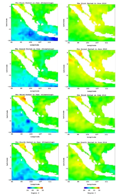
The climatological pattern of sea
surface temperature from the first to the
fourth pentad and in the western waters of Sumatra and the southern waters of Java in June 2016, is illustrated in Figure 5. The climatological mean of sea surface temperature in the southern waters of Java in June was lower than those in the western
waters of Sumatra. Climatological means
of sea surface temperature from the first to
the fourth pentad in BS1, BS2, and SJ were approximately 29.3°C, 28.4°C, and 27.9°C, respectively.
Sea surface temperature in the western waters of Sumatra and the southern waters
of Java from the first to the fourth pentad of
June 2016 showed an increasing trend. The anomalies of sea surface temperature in BS1 and BS2 were 0.9°C and 1.8°C, respectively. Meanwhile, the anomaly of sea surface temperature in SJ was 1.6°C. The highest anomaly of sea surface temperature in the western waters of Sumatra of 2.1°C occurred
in BS1 in the third pentad and in SJ in the first
The results indicated that the anomalies of sea surface temperature in the western waters of Sumatra and the southern waters of Java
during the first to the fourth pentad of June
2016 showed a positive value. It was indicated by the relatively high sea surface temperature in June 2016. Normally, in June, the sea surface temperature in the southern waters of Java to the south-west waters of Sumatra is cold due to the upwelling process. The position of the Sun in the northern hemisphere leads to the low air pressure in the northern hemisphere and the high air pressure in the southern hemisphere. It causes the formation of the Australia monsoon. At the same time, the south-east trade wind blows in the western waters of Sumatra and the southern waters of Java. The Australia monsoon and the south-east trade wind have the same direction, so they have mutual reinforcement.
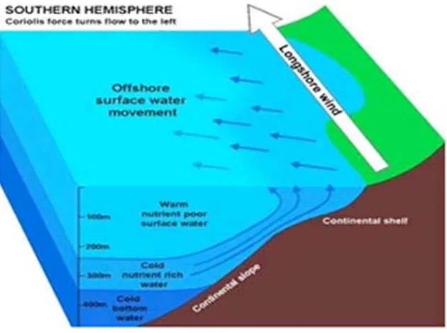
In June, surface wind in the southern waters of Java moves to the west. The stress of surface wind would push the surface water mass in the same direction with the wind to the west. Because it is located in the southern hemisphere, the movement of the water mass
will be deflected to the left at a 45° angle to
the wind direction and will form Ekman spiral. The net transport in the Ekman layer
will be deflected to the left at a 90° angle to
the wind direction. This condition will cause the surface water mass in the coastal waters to move towards offshore waters as shown in Figure 6. This mechanism caused sea level on the coast is lower than the offshore. In order to eliminate the sea level difference between the coast and the offshore, the water mass from the bottom layer will move to the surface. As a consequence, surface temperature in the coast is colder than the surrounding area.
Figure 6. Upwelling process in the southern waters of Java. Source: https://cmast.ncsu.edu
The analysis showed the anomaly of sea surface temperature in the western waters of Sumatera and the southern waters of Java increased from 1 – 20 June 2016. The rise of sea surface temperature was caused by the change of surface current due to extreme weather in those waters. In June, normally, the surface wind in BS1 moves to the northeast, in BS2 moves to the
Figure 7. The pattern of surface current in June, left (climatology) and right (2016).
Figure 8. Pattern of surface current from the first to the fourth pentad in June 2016.
Pattern of surface current in the western waters of Sumatera and the southern waters of
Java from the first until the fourth pentad of June
2016 is demonstrated in Figure 8. In this period, pattern change of surface current took place.
Current in the southern waters of Java shifted to the south up to 10°S. This mechanism caused surface current in the southern waters of Java from the coast of 10°S moved to the east. This pattern of surface current was contrast to the normal condition where the current moved to the west.
4. Conclusions
Based on the results, it can be concluded that extreme weather occurred in the western waters of Sumatra and the southern waters of Java in 1 – 20 June, 2016. Surface wind in the western waters of Sumatra moved to the south-east with higher intensity than the
normal condition. Extreme weather changed the pattern of surface current in the western waters of Sumatera that moved to the south-east as well as in the southern waters of Java that moved to the east. The change caused the lower upwelling intensity that led to the increase of sea surface temperature. The increases in BS1, BS2, and SJ were 0.9°C, 1.8°C, and 1.6°C, respectively.
5. Acknowledgements
Author would like to thank Center of Atmospheric Science and Technology for the
financial support in this research.
6. References
Aldrian, E. (2008). Meteorologi Laut Indonesia. Badan Meteorologi dan Geofisika, Jakarta.
Dahuri, R., Rais, J., Ginting, S.P., Sitepu, M.J. (1996). Pengelolaan Sumber Daya Wilayah Pesisir dan Lautan Secara Terpadu. Pradnya Paramita, Jakarta.
Ibrayev, R.A., özsoy, E., Schrum, C., Sur, H.I. (2010). Seasonal variability of the Caspian Sea three-dimensional circulation, sea level and air-sea interaction. Ocean Sci, 6: 311–329.
Kemili, P., and Putri, M.R. (2012). Pengaruh Durasi dan Intensitas Upwelling Berdasarkan Anomali Suhu Permukaan Laut terhadap Variabilitas Produktivitas Primer Di Perairan Indonesia. Jurnal Ilmu dan Teknologi Kelautan Tropis, 4(1): 66-79.
Kunarso, Ningsih, N.S., Supangat, A. (2005). Karakteristik Upwelling di Sepanjang Perairan Selatan NTT Hingga Barat Sumatera. Ilmu Kelautan, 10 (1): 17 – 23.
Kunarso, Hadi, S., Ningsih, N.S., Baskoro, M.S. (2011). Variabilitas Suhu dan Klorofil-a di Daerah
Upwelling pada Variasi Kejadian ENSO dan IOD di Perairan Selatan Jawa sampai Timor. Ilmu Kelautan, 16(3):171-180.
Martono, M. (2016). Seasonal and Inter Annual Variation of Sea Surface Temperature in the
Indonesian Waters. Forum Geografi, 30(2), 120–129.
Qu, T., Du, Y., Strachan, J., Meyers, G., Slingo, J. (2005). Sea Surface Temperature and Its Variability in The Indonesian Region, Oceanography, 18(4): 50-61.
Supari, Tangang, F., Juneng, L., & Aldrian, E. (2016a). Observed changes in extreme temperature and precipitation over Indonesia. International Journal of Climatology, n/a-n/a. https:// doi.org/10.1002/joc.4829
Supari, Tangang, F., Juneng, L., Aldrian, E., Ibrahim, K., Badri, K. H., Yaacob, W. Z. W. (2016b). Spatio-temporal characteristics of temperature and precipitation extremes in Indonesian Borneo. AIP Conference Proceedings, 1784(1), 060050. https://doi.org/10.1063/1.4966888 Supriatin, L. S., & Martono, M. (2016). Impacts of Climate Change (El Nino, La Nina, and Sea
Level) on the Coastal Area of Cilacap Regency. Forum Geografi, 30(2), 106–111.
Susanto, D., and Marra, J. (2005). Effect of the 1997/98 El Niño on Chlorophyll a Variability along the Southern Coasts of Java and Sumatra, Oceanography, 18(4): 124-127.
Shenoi, S.S.C., Saji, P.K., Almeida, A.M. (1999). Near-surface circulation and kinetic energy in the tropical Indian Ocean derived from Lagrangian drifters. Journal of Marine Research,
57:885–907.
Syafik, A., Kunarso., Hariadi. (2013). Pengaruh Sebaran Dan Gesekan Angin Terhadap Sebaran
Suhu Permukaan Laut Di Samudera Hindia (Wilayah Pengelolaan Perikanan Republik
Indonesia 573). Jurnal Oseanografi, 2(3):318-328.
Tjasyono, B. (2004). Klimatologi. Penerbit ITB, Bandung.
Wyrtki, K. (1961). Physical Oceanography of the Southeast Asian Waters. Naga Report Volume 2, Scripps Institution of Oceanography, California.
Yoga, R.B., Setyono, H., Harsono, G. (2014). Dinamika Upwelling dan Downwelling Berdasarkan