A process based diagnostic approach to m

A process-based diagnostic approach to model evaluation:

Application to the NWS distributed hydrologic model

Koray K. Yilmaz,1Hoshin V. Gupta,1 and Thorsten Wagener2

Received 29 November 2007; revised 12 May 2008; accepted 23 May 2008; published 11 September 2008.

[1] Distributed hydrological models have the potential to provide improved streamflow

forecasts along the entire channel network, while also simulating the spatial dynamics of evapotranspiration, soil moisture content, water quality, soil erosion, and land use change impacts. However, they are perceived as being difficult to parameterize and evaluate, thus translating into significant predictive uncertainty in the model results. Although a priori parameter estimates derived from observable watershed characteristics can help to minimize obstacles to model implementation, there exists a need for powerful automated parameter estimation strategies that incorporate diagnostic information regarding the causes of poor model performance. This paper investigates a diagnostic approach to model evaluation that exploits hydrological context and theory to aid in the detection and resolution of watershed model inadequacies, through consideration of three of the four major behavioral functions of any watershed system; overall water balance, vertical redistribution, and temporal redistribution (spatial redistribution was not

addressed). Instead of using classical statistical measures (such as mean squared error), we use multiple hydrologically relevant ‘‘signature measures’’ to quantify the performance of the model at the watershed outlet in ways that correspond to the functions mentioned above and therefore help to guide model improvements in a meaningful way. We apply the approach to the Hydrology Laboratory Distributed Hydrologic Model (HL-DHM) of the National Weather Service and show that diagnostic evaluation has the potential to provide a powerful and intuitive basis for deriving consistent estimates of the parameters of watershed models.

Citation: Yilmaz, K. K., H. V. Gupta, and T. Wagener (2008), A process-based diagnostic approach to model evaluation: Application to the NWS distributed hydrologic model,Water Resour. Res.,44, W09417, doi:10.1029/2007WR006716.

1. Introduction

[2] ‘‘Distributed’’ watershed models provide the potential

ability to simulate the spatial distribution of hydrologic processes over the landscape [Refsgaard and Storm, 1995; Ivanov et al., 2004; Carpenter and Georgakakos, 2004; Smith et al., 1995;Koren et al., 2004], as well as to provide estimates of discharge volume along the entire length of the channel network. As such they are important tools for improving our knowledge of watershed functioning, for providing critical information in support of sustainable management of water resources, and for mitigating water related natural hazards such as flooding. However, contro-versy regarding the use of distributed modeling persists [Beven, 1989, 2002; Grayson et al., 1992]. Their spatial complexity is perceived to be an obstacle to the proper identification of model components and parameters, trans-lating into significant predictive uncertainty in the model results [Beven and Freer, 2001].

[3] For distributed watershed models to realize their full

potential, it is necessary to develop improved data mining strategies and techniques for assimilating information from large spatiotemporal data sets. This includes the formulation of powerful and rigorous methods for testing the assumed structure of the model (structural consistency) and for evaluating its input-state-output behavior (behavioral con-sistency) [Gupta et al., 2008]. Recognizing this, the Dis-tributed Model Intercomparison Project (DMIP [Smith et al., 2004;Reed et al., 2004]) was organized by the Hydrol-ogy Lab of the National Weather Service (HL-NWS) to evaluate various strategies for distributed watershed model-ing, including the so-called ‘‘physics-based-distributed’’, ‘‘conceptual-distributed’’, and ‘‘conceptual-semidistributed’’ approaches, in terms of their power and usefulness for operational water resources management and hazard miti-gation. A major conclusion of the first phase of this study (DMIP-1 [Smith et al., 2004]) was that the potential benefits of distributed models for operational use have yet to be realized, and that ‘‘reliable and objective procedures for parameter estimation, data assimilation, and error correc-tion’’ still need to be developed.

[4] An important strength of distributed watershed

mod-els is the potential ability to infer model parameter values directly from spatiotemporal data, by establishing ‘‘physical’’ or ‘‘conceptual’’ relationships between observable 1_{Department of Hydrology and Water Resources, University of Arizona,}

Tucson, Arizona, USA.

2_{Department of Civil and Environmental Engineering, Pennsylvania} State University, Pennsylvania, USA.

Copyright 2008 by the American Geophysical Union. 0043-1397/08/2007WR006716$09.00

W09417

Here

for

watershed characteristics (e.g., geology, topography, soils, and land cover, etc.) and the parameters for the hydrological processes represented in the model [e.g., see Refsgaard, 1997;Woolhiser et al., 1990;Koren et al., 2000; Leavesley et al., 2003]. However, difficulties can arise when param-eters defined using relationships based in ‘‘small-scale’’ hydrological theory are embedded in larger-scale model grids without proper account for heterogeneity, emergent process-es, scaling, and interactions across scales. An increasing body of literature suggests that ‘‘a priori’’ parameters derived in this way may need to be refined through an adjustment process to ensure proper consistency between the model input-state-output behavior and the available data [Gupta et al., 1998; Madsen, 2003; Reed et al., 2004]. While it is possible (and desirable) that this step will eventually become unnecessary, the current reality is that even the most sophis-ticated hydrological models require parameter adjustments to meet the needs of operational decision making.

[5] A variety of parameter adjustment (model calibration)

techniques are being applied to the problem of improving the behavioral performance of distributed watershed mod-els, by assimilating information from a variety of different data sources [Madsen, 2003; Leavesley et al., 2003; P. Pokhrel et al., A spatial regularization approach to param-eter estimation for a distributed watershed model, submitted to Water Resources Research, 2008] using multicriteria approaches [Gupta et al., 1998; Yapo et al., 1998; Boyle et al., 2000;Wagener et al., 2001;Vrugt et al., 2003, etc.]. However, it is still not yet well understood how to provide an adequate basis for diagnosing the causes of model performance inadequacies and to provide meaningful guid-ance toward improving the model [Gupta et al., 2008]. The main reasons for this include the lack of (1) objective and robust model performance evaluation criteria that have diagnostic power (i.e., that point toward the causes of the poor performance), and (2) systematic procedures for mak-ing appropriate model improvements (to parameters and/or structure) that improve the overall consistency, accuracy and precision of model performance.

[6] The goal of this paper is to discuss the problem of

diagnostic evaluation in the context of watershed models, and to develop a procedure for adjusting the spatially distributed a priori parameter estimates of the Hydrology Laboratory Distributed Hydrologic Model (HL-DHM) of the National Weather Service (NWS) so as to improve its overall performance in a hydrologically meaningful manner. Section 2 sets the context for this work, and describes the study area, data, HL-DHM model and the methodology for estimating a priori values of its parameters. Section 3 provides an evaluation of the baseline performance of the HL-DHM model. Sections 4, 5 and 6 discuss our diagnostic model evaluation strategy and its application to the HL-DHM model. Section 7 presents a discussion of the study conclusions and our suggestions for future work.

[7] Please note that the diagnostic approach presented

here is general and applicable to any watershed model (including physics based models), although the actual interpretations of the diagnostic information will vary from model to model. This being an initial investigation, our primary focus will be on overall model performance at the outlet, and not on its distributed response. Further, we will assume that sufficient a priori information exists to

ade-quately characterize the spatial patterns of the parameter fields in a relative sense. Future work will build a more comprehensive strategy by progressively relaxing the assumptions incorporated here.

2. Context for the Study

[8] Successful implementation of a spatially distributed

hydrologic model requires the following steps, in each of which there remains considerable room for improvement:

[9] 1. Model Conceptualization: Development of a clear

perceptual and conceptual understanding of the basin char-acteristics and processes that control its hydrological input-state-output behavior. Every simplifying assumption in this process should be explicitly stated.

[10] 2. Development of Numerical Model: Formulation of

a mathematical model structure consistent with the concep-tual model identified in step one, and numerical implemen-tation of the model using computer code.

[11] 3. A Priori Estimation of Parameters: Development

of a strategy for a priori specification of (spatially distrib-uted) model-parameter fields from observable watershed data regarding geology, soils, topography, and land cover etc. Where such specification is subject to significant uncertainties, the range (or distribution) of uncertainty should be given.

[12] 4. Performance Assessment and Diagnostic

Evalu-ation: Specification of an objective and robust procedure for diagnostic evaluation of model performance via com-parison of its input-state-output behavior to observations of various kinds that are related to the dynamic response of the watershed.

[13] 5. Model Improvement: Development of a

system-atic procedure for making model improvements (to param-eters and/or structure) so as to improve the overall consistency, accuracy and precision of model performance. [14] In the work reported here we assume that a suitable

conceptual/numerical model for the selected study area is already available (the HL-DHM model; see section 2.2), along with a suitable strategy for a priori estimation of spatially distributed fields of parameter values (theKoren et al.[2000], approach; see section 2.3). Our study area is the Blue River Basin located in southern Oklahoma and used in both phases One and Two of the DMIP study. We seek to develop objective and systematic strategies for model per-formance assessment that support and enable a diagnostic approach to detection and resolution of model inadequacies, and that lead to clear improvements in its predictive accuracy.

2.1. Study Area and Data

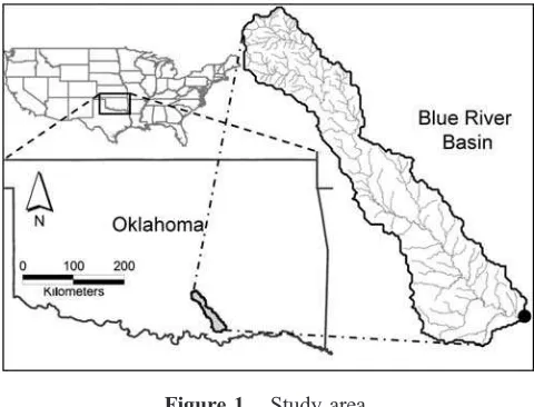
[15] The Blue River Basin (outlet at USGS Streamgage

[16] Data for the time period 10/1996 – 9/2002 (6 years) is

available from the DMIP-2 website (http://www.nws.noaa. gov/oh/hrl/dmip/2/index.html) including: (1) hourly stream-flow observations at the outlet, (2) 4 km 4 km gridded hourly precipitation estimates (radar/gage merged) and (3) 4 km 4 km gridded mean monthly potential evaporation estimates. The latter are converted to potential evapotrans-piration (hereafter NWS-PET) by multiplying them with a gridded land cover correction factor (also provided by NWS). Furthermore, USGS daily streamflow data for the period of 10/2002-9/2006 is used for testing the diagnostic approach (section 6).

2.2. The HL-DHM Model

[17] The HL-DHM is a hybrid conceptual-physical

dis-tributed watershed model consisting of the Sacramento soil moisture accounting model (SAC-SMA [Burnash et al., 1973; Burnash, 1995]) applied over a grid consisting of regular 4 4 km spatial elements, linked to a kinematic wave model for hill slope and channel network flow routing [Koren et al., 2004]. The vertical soil column is represented conceptually using two zones; the upper zone represents near-surface soil moisture storage and mediates the process-es of surface interception, evapotranspiration, infiltration and lateral flow, and the lower zone accounts mainly for longer-term groundwater storage and release. Each zone represents both ‘‘tension water’’ (moisture bound to the soil particles) removable only by evapotranspiration and ‘‘free water’’ (which can move both horizontally and vertically in response to gravity). By representing two kinds of free water in the lower zone, the model can simulate multirate hydrograph recessions. Water percolates from the upper to lower zones via a complex dependence on the availability of water in both zones. Other behaviors include the effects of time-variable impervious area sizes and of evapotranspira-tion by riparian vegetaevapotranspira-tion. The grid-scale response to spatially distributed precipitation is computed by routing the ‘‘fast’’ runoff response (impervious, surface and direct runoff) to the nearest stream channel via kinematic hill-slopes, and the ‘‘slow’’ runoff response (interflow and baseflow) directly to the nearest stream channel. The routing parameters (Table 1) for the study area were obtained from the DMIP-2 website. The model was run using an hourly time step (except in section 6 where a daily time step was used), driven by gridded estimates of

precip-itation and evapotranspiration demand. The model output consists of streamflow along the channel and estimates of soil moisture and evapotranspiration at each element.

2.3. A Priori Parameter Estimates

[18] Sixteen soil moisture accounting parameter fields,

3 kinematic wave hill slope routing parameter fields, and 2 kinematic wave channel routing parameter fields must be specified for every 4 km x 4 km element over the study domain (Table 1). As discussed byDuan et al.[2001] and Koren et al.[2000, 2003, 2004], the formulation of the HL-DHM model is consistent with observations of the soil moisture profile obtained via experimental studies such as those byGreen et al.[1970] andHanks et al.[1969].Koren et al. [2000] exploited this fact in the development of a general approach by which the parameters of conceptual multilayer hydrological model parameters can be estimated from soils and vegetation data. The model storage compo-nents are related to soil hydraulic properties by assuming that the ‘‘tension water capacity’’ corresponds to soil available water (the difference between field capacity and wilting point) and the ‘‘free water capacity’’ corresponds to soil gravitational water (the difference between porosity and field capacity). Similarly, other parameters, including lateral soil drainage and vertical percolation rates, are related to the hydraulic properties of the soil. For the two-layer HL-DHM conceptualization, the Koren a priori estimation approach implements a combination of physically based and empir-ically derived relationships to develop spatially consistent a priori estimates for 11 of the model parameters. The remaining 5 SAC-SMA parameters are set to nominal values based on previous NWS experience with lumped implementation of the model over the US. For details, please refer to Koren et al. [2000, 2003], Duan et al. [2001], and Anderson et al. [2006]. Spatially distributed parameter fields derived for the Blue River Basin from STATSGO soils data using the Koren approach can be downloaded from the DMIP-2 website.

3. Preliminary Evaluation of the Baseline Model [19] The first step in model evaluation is to detect and

resolve major inconsistencies in the initial model setup. If inconsistencies in the input-state-output data sets (Precipi-tation, PET, Streamflow, and Initial state values) are not removed, they will undermine subsequent efforts toward model identification. Having specified a priori parameter estimates for the HL-DHM model of the Blue River Basin using the Koren approach, this ‘‘baseline’’ model was used to generate input-state-output simulations for the six-year period 10/1996 – 9/2002. Various diagnostic plots and com-putations were then used to examine the model behavior, as discussed below.

3.1. A Check on the Specification of Initial State Values

[20] The distributed HL-DHM model requires

specifica-tion of initial water content for six storage capacities (3 for the upper zone and 3 for the lower zone; see Table 1) for every element within the study area. In the absence of information about the spatial distribution of soil moisture content, these initial values are usually set to fixed fractions of the respective water holding capacities, reflecting typical dry conditions at the end of September; in our case

UZTWC/UZTWM = 0.1, UZFWC/UZFWM = 0.14, LZTWC/LZTWM = 0.1, LZFSC/LZFSM = 0.11, and LZFPC/LZFPM = 0.1 and ADIMC = 0 (Table 1). While these values represent ‘‘reasonable’’ guesses regarding the initial soil moisture conditions, it might be expected that the effects of errors in their specification would become min-imal over some reasonable length of ‘‘spin-up’’ time, particularly if the climate of the watershed goes through an extreme period (dry or wet). The integral form of the continuity equation:

represents the time evolution of water balance of the model, where Xt is the total water accumulated within all the storages of the model (the overall model ‘‘state’’),Xois the initial water storage, PtandETtare total areal precipitation and evapotranspiration over the watershed, and Qt is the watershed outlet streamflow, all at timet(we assume that all of the groundwater flow contributes to streamflow discharge at the outlet and there is no loss to deep percolation). Over the long term, and under stationary climate conditions, the

changes in storage DX should vary seasonally around a steady state value of zero, becoming negative during hot dry months and positive during the cooler wetter months.

[21] Figure 2 (dashed line-circle) shows the time

evolu-tion of cumulative change in model state,DXsim, obtained by substitutingQsimandETsim(computed using the baseline model) as well as Pobs (observed precipitation) into equation (1). The figure reveals that the model absorbs a rather large amount of water during the first month (October 1996; DXsim jumps from 0 to 85 mm) before settling down to vary in a periodic seasonal manner around the mean value of +108 mm. Further, a comparison of observed and simulated monthly streamflow (figure not shown) shows that the model has strongly underestimated observed streamflow for the first month by as much as 47%. This suggests that the model has been incorrectly initialized to state values that are too dry for the specific hydroclimatol-ogy of the Blue River Basin. Correct initialization should result inDXsimvarying (over the long term) around a mean close to zero, with little or no bias in monthly estimation of streamflow during the early portion of the study period.

[22] To develop better initial estimates for the model state

variables, the input-output data were carefully examined to

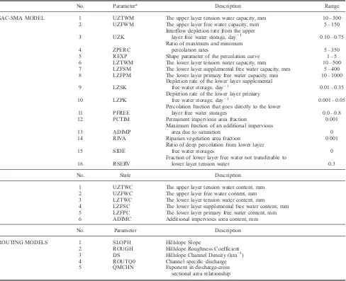
Table 1. Parameters of the HL-DHM Model

No. Parametera _{Description Range}

SAC-SMA MODEL 1 UZTWM The upper layer tension water capacity, mm 10 – 300 2 UZFWM The upper layer free water capacity, mm 5 – 150

3 UZK

Interflow depletion rate from the upper

layer free water storage, day1 _{0.10 – 0.75}

4 ZPERC

Ratio of maximum and minimum

percolation rates 5 – 350

5 REXP Shape parameter of the percolation curve 1 – 5 6 LZTWM The lower layer tension water capacity, mm 10 – 500 7 LZFSM The lower layer supplemental free water capacity, mm 5 – 400 8 LZFPM The lower layer primary free water capacity, mm 10 – 1000

9 LZSK

Depletion rate of the lower layer supplemental

free water storage, day1 0.01 – 0.35

10 LZPK

Depletion rate of the lower layer primary

free water storage, day1 _{0.001 – 0.05}

11 PFREE

Percolation fraction that goes directly to the lower

layer free water storages 0.0 – 0.8 12 PCTIM Permanent impervious area fraction 0.001

13 ADIMP

Maximum fraction of an additional impervious

area due to saturation 0

14 RIVA Riparian vegetation area fraction 0.001

15 SIDE

Ratio of deep percolation from lower layer

free water storages 0

16 RSERV

Fraction of lower layer free water not transferable to

lower layer tension water 0.3

No. State Description

1 UZTWC The upper layer tension water content, mm 2 UZFWC The upper layer free water content, mm 3 LZTWC The lower layer tension water content, mm

4 LZFSC The lower layer supplemental free water content, mm 5 LZFPC The lower layer primary free water content, mm 6 ADIMC Additional impervious area content, mm

No. Parameter Description

ROUTING MODELS 1 SLOPH Hillslope Slope

2 ROUGH Hillslope Roughness Coefficient 3 DS Hillslope Channel Density (km1) 4 ROUTQ0 Channel specific discharge 5 QMCHN Exponent in discharge-cross

sectional area relationship

a

find a time period having rainfall and flow conditions similar to the initial time period. The date October 10, 2001 at the beginning of the sixth water year was selected and the average fractional water contents for the five model storages simulated for that time by the baseline model run were computed (UZTWC/UZTWM = 0.81; UZFWC/ UZFWM = 0.006; LZTWC/LZTWM = 0.55; LZFSC/ LZFSM = 0.10; LZFPC/LZFPM = 0.47; ADIMC = 0). After re-setting the model initial soil moisture contents to these values, assuming uniform application across all the elements, the recomputed time evolution of cumulative DXsim now varies seasonally around a mean value close to zero (Figure 2, solid line-circle); further, the model flow bias for the first month has reduced from 47% to a more acceptable 3% (not shown).

3.2. A Check on the Specification of Potential Evapotranspiration

[23] We next examine the data to detect any significant

errors that may affect the baseline model performance. Evapotranspiration, a major component of the water balance in most catchment studies, cannot be measured directly and is frequently a principal source of error in hydrologic prediction [Morton, 1983;Vorosmarty et al., 1998;Vazquez and Feyen, 2003]. While evapotranspiration can affect the water balance (and shape of the hydrograph) at various timescales, e.g., evapotranspiration has a feedback mecha-nism with infiltration at short time scales—its major role is to control the long-term water balance.

[24] To assess the long-term behavior of the baseline

model we examine the annual plots (Figure 3) and the monthly cumulative plot (not shown) of the major water balance components (precipitation, flow and evapotranspi-ration), and note that the baseline model simulation (QSIM) consistently overestimates the observed flows (QOBS) with a 48% bias at the end of the 6-year period (Table 2). This tendency to overestimation is particularly significant for the years 1999 and 2000, which are characterized by very low

flows. This problem could be caused by some combination of large positively biased errors in precipitation, large negatively biased errors in potential evapotranspiration (PET), and/or unaccounted groundwater losses from the basin. In the absence of further information we follow the DMIP study assumption that the last factor can be ignored. Further, since the precipitation data has already undergone some degree of quality control, and since a positive 48% bias in the precipitation data seems unlikely, we turn our attention to the PET data. From Figure 3a we note that the DMIP data set prescribes a pattern of annual PET that remains constant over the years. Given the actual pattern of interannual climatological variation indicated by variation in annual ‘‘wetness’’ (i.e., precipitation) this assumption of annually repeating NWS-PET sequence seems unreason-able, and is a likely major reason for some of the positive bias in simulated runoff.

[25] An alternative PET data set is provided by the North

American Regional Reanalysis (NARR), based on a com-putation that is designed to be internally self-consistent from a hydroclimatological standpoint [Mesinger et al., 2006]. Figure 3 shows that the NARR-PET is consistently and significantly larger (20 – 70%) than the NWS-PET and varies in a manner that is climatologically more consistent with the variation in observed annual precipitation. Rerun-ning the baseline model using NARR-PET estimates [see Yilmaz, 2007, for details] we see that the overall bias has been reduced to 19% (Table 2), and that the simulated annual flows (Figure 3b) now follow the observations more closely. Here-after ‘‘baseline model’’ refers to the HL-DHM model with a priori parameters specified via the Koren et al. [2000] approach and using the NARR-PET data set described above.

4. The Diagnostic Model Evaluation Approach [26] At this point, significant bias still remains in the

baseline model simulation of the flows, and we are faced

with a sort of ‘‘chicken-egg’’ model evaluation problem. The remaining biases could be caused by numerous factors including remaining problems in specification of the initial states and problems in the precipitation and PET data, or could be a result of incorrect model parameterization. Although we could now cycle back through the input-state-output and data checking procedure followed above, we will instead proceed under the assumption that the major cause of this remaining bias is incorrect specification of the model parameter fields. The problem is to diagnose which parameter fields have been incorrectly specified and are largely responsible for the observed biases in model input-state-output performance. The classical approach is to simultaneously adjust all (or most) of the parameter fields so as to optimize some overall aggregate measure of model fit to the data [e.g.,Duan et al., 1992]. Many problems arise with this approach, including the well-known fact that, if not careful, we can achieve improved model performance for the wrong reasons. The idea of a ‘‘diagnostic’’ approach is to attempt to minimize this kind of problem.

4.1. The Basis for a Diagnostic Approach

[27] Model diagnosis is a process by which we make

inferences about the possible causes of an observed unde-sirable symptom via targeted evaluations of the input-state-output response of the system model. For a model evalua-tion strategy to have diagnostic power, it must be capable of highlighting inadequacies in model performance, and also of pointing (in a meaningful way) toward the specific aspects of the model structure (model components) and/or parameterization that are causing the problem(s). As dis-cussed by Gupta et al. [1998, 2008] and Wagener and Gupta [2005], automated model evaluation strategies that rely on the use of a single regression-based aggregate measure of performance (e.g., Mean squared error or the corresponding normalized Nash Sutcliffe efficiency) are, in general, weak at the task of simultaneously discriminating between the varied influences of multiple model compo-nents or parameters on the model output. A major reason is the loss (or masking) of valuable information inherent in the process of projecting from the high dimension of the data set (<Data) down to the single dimension of the residual-based summary statistic (<1

), leading to an ill-posed pa-rameter estimation problem (<Parameter <1) [Gupta et al., 2008]. Therefore a diagnostic evaluation strategy must necessarily make use of multiple, carefully selected, meas-ures of model performance, more closely matching the number of unknowns (the parameters) with the number of pieces of information (the measures), thereby resulting in a better-posed identification problem.

[28] In this regard, it is useful to note that the traditional

interactive process of manual-expert calibration effectively follows a powerful (albeit somewhat subjective) multicri-teria approach wherein a variety of graphical tools and numerical measures are used to target different aspects of model response [Boyle et al., 2000; Smith et al., 2003; Bingeman et al., 2006], which are then subjectively related to possible model related causes (model components, parameters, initial states, and data) by reference to an accumulated body of knowledge. A number of hybrid model evaluation strategies have sought, with varying degrees of success, to combine the important strengths of manual and automatic model evaluation [Brazil, 1988; Harlin, 1991; Zhang and Lindstro¨m, 1997; Boyle et al., 2000;Leavesley et al., 2003;Turcotte et al., 2003].

[29] Following in these footsteps, the core of our strategy

is a hierarchical focus on the primary functions of any watershed and their representation in the water balance

Figure 3. Annual variation of major water balance components (a) using NWS-PET and (b) using NARR-PET (POBS = observed precipitation; QOBS = Observed flow; QSIM = Simulated flow; ETSIM = Simulated evapotranspiration; PET = Potential Evapotranspiration).

Table 2. Summary of Modeled Flow Statistics (%DIndicates the Percent Change From the Observed Value)

Flow Statistics Observed

Baseline (NWS-PET) (%D)

Baseline (NARR-PET) (%D)

Mean (mm/hr) 0.027 +48 +19

Variance 0.008 +13 19

Skewness 8.74 12 8

Mean (Log) 2.05 +14 +9

Variance (Log) 0.327 27 28 Skewness (Log) 0.233 +329 +349 Flow Groups

High 0.105 +43 +15

Medium 0.011 +62 +26

computations of a model. For example, Wagener et al. [2007] identified the three basic watershed functions as being: partition, storage and release. Similarly, Black [1997] suggested three hydrological functions (collection, storage and discharge) and two ecological functions (chem-ical and habitat) of a watershed. Our interest, however, is in the extraction of diagnostic information from watershed input-state-output observations—i.e., we seek representa-tions for which the functionality can be detected and some-how quantified from the data. We therefore characterize the four primary functions of a watershed system (Figure 4) in a time-hierarchical sense, as being to: (1) maintain overall water balance, (2) vertically redistribute excess rainfall between the faster and slower runoff components, (3) redis-tribute the runoff in time (influencing hydrograph timing and shape), and (4) redistribute the moisture in space.

[30] With this focus, the critical task is to design

‘‘diag-nostic’’ measures that are definable using available obser-vations on input-output data, capable of extracting useful information pertaining to system functioning, and capable of discriminating between the varied influences of multiple model components or parameters. Clearly this task can only be pursued in the context of the hydrological theory that underlies the model to be evaluated [Gupta et al., 2008].

[31] A natural way to look for relevant hydrological

information in the data is to focus on the spatiotemporal patterns that can be related to specific hydrological processes acting on the watershed [Grayson and Bloschl, 2000]. Therefore the basis for developing a diagnostic approach to model evaluation lies in the detection of characteristic or ‘‘signature’’ patterns in the input-output data and in relating these to their causal mechanisms. For example, the top-down approach to model development seeks to start with the simplest model possible, and uses signature patterns in the data to progressively increase the model structural complexity in ‘‘direct response to demonstrated deficiencies in the model prediction’’ [Atkinson et al., 2002], until a desired level of model accuracy is achieved [see also Klemes, 1983; Sivapalan et al., 2003; Jothityangkoon et al., 2001; Atkinson et al., 2003; Fenicia et al., 2008]. However, while these authors discuss the use of signature patterns in a diagnostic context, they continue to use classical residual based measures (e.g., Mean squared error, Correlation coefficient, etc.) to quantitatively characterize model performance. We argue that it is both necessary and important to actually formulate quantitative representations of these patterns in the form of ‘‘signature indices’’ that summarize the relevant and useful diagnostic information present in the data. If properly rooted in hydrologic context,

‘‘signature measures’’ computed from these indices can be used to facilitate the semiautomated detection of model failures, point toward possible causes, and guide plausible improvement strategies. Such measures must be constructed so as to quantify the manner in which signature index values computed from the model simulations differ from that of the observations. An important point is that signature measures are inherently different from classical optimization criteria in the sense that they point toward the direction of model improvements (i.e., can take positive and negative values while seeking a value of zero).

[32] The diagnostic approach is, therefore, to (1) identify

signature patterns of behavior that are related to the primary watershed functions and detectable using observed precip-itation-runoff data, (2) extract diagnostic signature indices related to these patterns/behaviors (3) test the ability of the watershed model to reproduce these signature indices, (4) detect and group together model components/parameters demonstrably related to each signature index (and therefore related system/model function), and (5) resolve signature index match failures via modifications to the associated model component/parameter group.

[33] Note that evaluating the correctness of a model’s

ability to represent the spatial distribution of processes, states and fluxes (as opposed to its overall aggregate behavior) is not the immediate focus of this paper; instead, we assume that the conceptual model structure and a priori estimates of the parameters reflect the spatial heterogeneity of the study basin in a realistic way.

4.2. Selection of the Signature Measures

[34] In implementing our diagnostic approach, we exploit

the well-known fact that processes related to different watershed/model functions exhibit dominance at a hierarchy of time scales [Klemes, 1983] to improve system observ-ability. In principle, model components and parameters that control the overall water balance can be evaluated using indices related to characteristic watershed behavior at longer time scales (study period, annual), while indices related to characteristic behaviors at shorter timescales can be used to evaluate model components/parameters related to vertical redistribution of water (e.g., partitioning among slow and fast runoff processes) and flow timing.

4.2.1. Signature Measure Related to Overall Water Balance

[35] We first seek a signature measure that can evaluate

and diagnose violations in the overall water balance func-tion of the system. Accepting the assumpfunc-tion that all infiltrated water contributes to streamflow at the outlet of the Blue River Basin, we require that a strict balance between the inputs (precipitation), storage (soil moisture), and outputs (evapotranspiration and runoff) be maintained via the continuity equation. A number of different quanti-tative and graphical indices are in common usage for characterizing the long-term input-output behavior for any watershed [e.g., runoff ratio and Budyko curve; Budyko, 1974]. Indices that focus on water-balance over the long term (e.g., annual) will be primarily sensitive to the climatic variability of evapotranspiration while showing only sec-ondary (or minimal) sensitivity to processes operating at shorter time scales. In this study we use the percent bias in overall runoff ratio (%BiasRR) as a diagnostic signature measure of system water balance (see Appendix A). This

measure is expected to show primary sensitivity to model parameters that control evapotranspiration.

4.2.2. Signature Measures Related to Vertical Soil Moisture Redistribution

[36] We next seek a signature measure sensitive to the

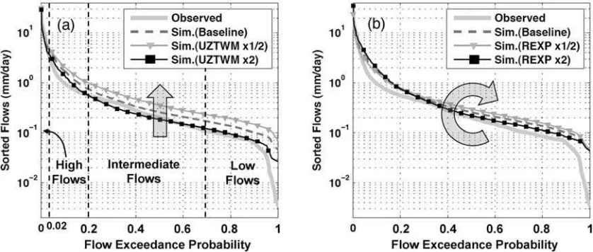
vertical redistribution, via percolation, of excess precipita-tion within the soil profile. The effects of this vertical redistribution are seen in the streamflow hydrograph as ‘‘fast’’ and ‘‘slow’’ runoff processes associated with imper-vious area runoff, surface runoff, interflow, and primary and secondary baseflow. The flow duration curve [(FDC) see Vogel and Fennessey, 1994, and Smakhtin, 2001], perhaps more accurately referred to as the flow exceedance proba-bility curve and commonly used to indicate and classify watershed functioning, summarizes a catchment’s ability to produce flow values of different magnitudes, and is there-fore strongly sensitive to the vertical redistribution of soil moisture within a basin, while being relatively insensitive to the timing of hydrologic events.

[37] To characterize the information in an FDC we

subjectively partition the curve into three different segments (Figure 5) and examine the properties; 1) high-flow segment (0 – 0.02 flow exceedance probabilities) characterizing wa-tershed response to large precipitation events, 2) midseg-ment (0.2 – 0.7 flow exceedance probabilities), characterized by flows from moderate size precipitation events and also related to the intermediate-term primary and secondary base flow relaxation response of the watershed, and 3) low-flow segment (0.7 – 1.0 flow exceedance probabilities), related to long-term sustainability of flow and controlled by the interaction of baseflow with riparian evapotranspiration (ET) during extended dry periods. A characteristic signature behavior for a watershed having ‘‘flashy’’ response (due to small soil storage capacity and hence larger percentage of overland flow) is a steep slope of the midsegment FDC, while flatter midsegment slopes are associated with water-sheds having slower and more sustained groundwater flow response. We therefore explore the use of the slope (rota-tion) of the FDC midsegment as a signature index of vertical redistribution of soil moisture. We also found (through empirical analysis) that the volume of water allocated to

the high flow segment is useful for this purpose; of course the FDC can also provide information related to the other functions of a watershed system (see Figure 5 and section 6). Therefore the diagnostic vertical redistribution signature measures used in this study are the percent bias in FDC midsegment slope (%BiasFMS) and the percent bias in FDC high-segment volume (%BiasFHV).

4.2.3. Signature Measure Related to Behavior of Long-Term Baseflow

[38] As mentioned above, the low-flow segment of the

FDC contains information related to long-term sustainabil-ity of flow and is controlled by the interaction of baseflow with riparian ET during extended dry periods (particularly in the Blue River Basin). Using the total volume of the low-flow segment as an index of long-term baselow-flow response, we define the diagnostic long-term baseflow signature measure to be the percent bias in FDC low-segment volume (%BiasFLV); note that we compute the ‘‘volume’’ after taking a log transform of the flows, to increase sensitivity to the very low flows.

4.2.4. Signature Measure Related to Timing

[39] Once the watershed model parameter fields are

con-strained to regions of the parameter space giving acceptable water balance and vertical redistribution of soil moisture, we can attempt to reproduce the timing of flows at finer time scales. Measures commonly used to evaluate the hydro-graph timing during automated parameter search are the ‘‘correlation coefficient between observed and simulated flows’’ [Fenicia et al., 2008] and the ‘‘bias in peak-flow timing’’ [Yilmaz et al., 2005;Yang et al., 2004]. Our notion of ‘‘diagnostic measures’’ favors indices easily and automati-cally computable from commonly available data sets while being indicative of intrinsic characteristics of a watershed (such as response time). We are therefore interested in an index relating the timing of the system output (flow) to that of its corresponding dominant driving flux (precipitation).

[40] One commonly used index of watershed timing is the

lag time between the centers of mass of ‘‘effective rainfall’’ and ‘‘direct runoff’’ [e.g., Simas, 1996] computed on a storm event basis. However, such computations, involving the partitioning of the data into individual storm events,

involve a level of difficulty and subjectivity that we seek to avoid in the development of automated identification pro-cedures. Instead, a simple way to characterize the mean rainfall-runoff lag time is to compute the time shift at which the cross-correlation between the mean areal rainfall and streamflow time series is maximized. While the use of a correlation coefficient is not strictly appropriate (it involves the implicit assumption that the watershed behaves like a linear system), the computational simplicity and correspon-dence to the concept of a watershed ‘‘lag time’’ makes it attractive as a diagnostic index of timing. We further extend this idea by including only times for which the flows are above a threshold flow level, easily selected by examination of the observed hydrograph. This has two main advantages: (1) it is likely that the linearity in the rainfall-runoff transformation increases with storm intensity [Caroni et al., 1986]; and (2) the high flows are more representative of direct runoff. Therefore the diagnostic timing signature measure used in this study is the percent bias in watershed lag time (%BiasTLag) above a selected flow threshold.

5. Diagnostic Evaluation of the HL-DHM Model Parameters

[41] We next test this suite of signature indices for

validity and diagnostic usefulness via a one-parameter-at-a-time perturbation analyses. Proceeding under the hypoth-esis that the a priori parameter estimates derived via the Koren approach (Table 1) provide a reasonable initial representation of the spatial heterogeneity of hydraulic properties in the Blue River Basin, we impose that spatial pattern as a constraint and perturb each parameter field using a multiplier (assuming monotonicity of the measure over multiplier interval); the parameter fields defining soil storage capacities are varied between 50% and 200% of their a priori values, the parameter fields defining drainage rates are varied to halfway between their a priori values and the upper and lower feasible limits (to maintain physical meaning), and the lumped riparian vegetation parameter RIVA is increased to 10 and 20 times its a priori value (0.001) to be able to examine its effect on the simulated flows. Of the routing parameters, only the channel specific discharge (ROUTQ0) is varied, to 73% and 117% of its a priori prescribed value, based on analysis of USGS dis-charge-area measurements [see Yilmaz, 2007].

[42] Figure 6a shows the sensitivity of %BiasRR to

variations in the parameter fields; the dashed-dotted line represents the baseline simulation with a positive +19% runoff ratio bias. The triangle and square markers indicate decreased and increased parameter values, respectively (perturbation magnitudes given in the paragraph above; note that the value of parameter RIVA was increased in both perturbations). The index is strongly sensitive to variations in parameters UZTWM, LZTWM and PFREE; this makes sense because parameters UZTWM and LZTWM control the amount of soil water capacity devoted to ‘‘tension’’ storage while PFREE controls the fraction of percolated water allocated between lower zone free and tension storages (tension storage regulates the amount of water available for ET). Increasing either or both UZTWM and LZTWM will increase the amount of water immediately available for ET and help to reduce the error in volume balance, while increasing PFREE will increase the volume

balance error by having the opposite effect. Parameters REXP, ZPERC, LZFSM, and LZSK (which control lower zone processes via percolation and baseflow) also have some (albeit smaller) effect on the overall water balance through indirect effects on the overall opportunity for ET loss from the lower zone. While such interacting (second-ary) effects can be unavoidable due to conceptual design of the model [seeGupta and Sorooshian, 1983], an important goal of signature measure selection is to minimize them as much as possible.

[43] Figure 6b shows the sensitivity of %BiasFMS to

perturbations of the parameter fields. The baseline run shows a negative (9%) bias, the measure is strongly sensitive to parameter LZFPM and somewhat sensitive to parameters REXP, UZFWM, ZPERC and PFREE. These parameters all influence vertical soil moisture redistribution via percolation and medium-term baseflow recession. Re-ducing LZFPM will help to reduce the error in FDC slope, by reducing the amount of percolation demand.

[44] Figure 6c shows the sensitivity of %BiasFHV to

perturbations of the parameter fields. The baseline run underestimates the high flows (14%), and the measure is primarily sensitive to parameters REXP and LZFSM and secondarily sensitive to LZTWM, LZFPM, LZSK, ZPERC. These parameters all influence percolation to the lower zone; smaller values (triangle markers) generally result in increased opportunity for high flows.

[45] Figure 6d shows the sensitivity of %BiasFLV to

perturbations of the parameter fields. The baseline run shows a strong positive bias (+70%), and the measure is most strongly sensitive to parameters RIVA (the fraction of watershed containing riparian vegetation, therefore control-ling demand for ET due to riparian vegetation) and LZPK (which controls the rate of primary baseflow recession). Increasing RIVA and/or LZPK will help to reduce bias in the FDC low-segment volume.

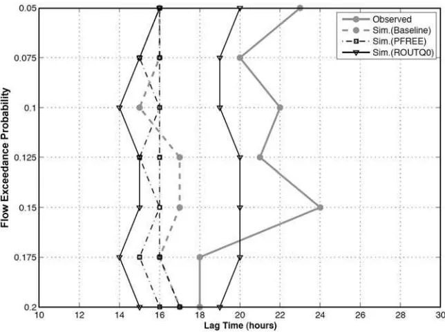
[46] Figure 7 shows the lag time computed for the hourly

time step using flow thresholds set at exceedance probabil-ity levels of 0.05, 0.075, 0.1, 0.125, 0.15, 0.175 and 0.2. We see that the observed lag time (gray-solid line-circle) varies between 18 and 24 hours while the baseline simulation of lag time (gray-dashed line-circle) varies between 15 and 17 hours, indicating that the characteristic response of the model is too quick. Also, the observed lag time is more variable for larger threshold values, probably because the real watershed system is more complex than the model representation (including e.g., that the precipitation data may not adequately characterize the true precipitation field). The perturbation analysis indicates that the simulated flow lag time is strongly sensitive to the perturbations of the channel routing parameter ROUTQ0 (solid line-triangle) and of the parameter UZFWM (not shown) but relatively insen-sitive to perturbations of the percolation parameter PFREE (dashed-dotted line-square) and other model parameters (not shown). Decreasing ROUTQ0 will help to increase the simulated lag time to better match the observed value.

6. Parameter Adjustment via Constrained Search [47] The perturbation analysis presented in section 5

difficulty involved in trying to derive indices that are sensitive only to specific watershed functions; for our problem some amount of compensating (interaction) effect caused by secondary parameter sensitivity was found to be unavoidable using the measures selected in this study. To arrive at improved estimates for the model parameters, we therefore used a simple automated approach to search for parameter fields that provide improved model performance — in terms of the signature measures identified above — while explicitly allowing for the effects of parameter inter-action on the evaluation.

[48] The goal here is to identify parameter fields that

provide simulations of the observed watershed functions (as represented by the signature indices) that are better than those achieved by the baseline model. The approach is to progressively constrain the ranges of parameters that have been found to exert primary control on the signature indices. We will retain conceptual consistency by proceeding in a time-hierarchical manner from higher to lower levels (see section 4.1). Because the computational cost involved in running the distributed model at an hourly time step for a

large number of sampled parameter sets is significant and would only allow simulations for relatively short time periods, this portion of the study was conducted using a daily modeling time step; even so about 48 continuous hours of computational time were required to generate 1600 runs. At each sampled parameter set, the signature measures were examined to study the properties of the parameter-to-signa-ture measure relationships. These relationships were used to constrain the ranges of the parameters in a progressive manner.

[49] To ensure a more complete exploration of the

feasi-ble space of spatially distributed parameters we imple-mented a novel strategy as follows. For distributed parameter models it is common to preserve the pattern of relative spatial variation provided by the a priori parameter estimates, and to vary only the mean level of each parameter field, by using one ‘‘multiplier’’ per field. This approach creates problems when any of the individual values in each parameter field exceeds its specified (physically rea-sonable) bounds; either the parameter distribution must be truncated so that any values exceeding the range are fixed at

the boundaries (see case M = 1.9 in Figure 8), or the mean level must be prevented from varying over the entire range. An alternative, more flexible, approach that removes these restrictions can be achieved by using the nonlinear trans-formation:

qb_g¼qminþqmaxqmin

* q

p gq

min

qmaxqmin

!a

g¼1;2;. . .G ð2Þ

a¼log10 1 2b

2

log10ð0:5Þ

ð3Þ

whereGis the number of elements in the current parameter field, qp is the a priori parameter field, and qb is its corresponding adjusted value constrained by the transfor-mation to remain within the feasible parameter region [qmin,

qmax]. Here instead of varying a ‘‘multiplier’’, as in the conventional approach, we vary the value of the parameter field coefficientbon the range [0, 2]; whenb= 1 (hencea= 1) the transformed parameter field remains identical to the original a priori field (i.e.,qb=qp), whenb!0 (a! 1) the transformed parameter field approaches the lower bound, and whenb !2 (a!0) the transformed parameter field approaches the upper bound (Figure 8). Notice that asb is varied away from 1 towards either of its limiting values, the variance of theqbparameter distribution is compressed so as to keep the entire distribution within the feasible range while preserving the monotonic relative ordering of parameter values in the field.

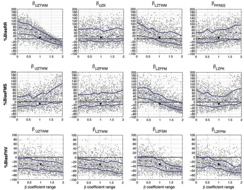
[50] Application of this nonlinear transformation results

in twelveb coefficients to be varied (11 SAC-SMA model

parameter fields, parameters 1 – 11 in Table 1, and the routing model parameter field ROUTQ0). We randomly generated 1600 model parameter fields using uniform sampling of the twelveb coefficients on the ranges (0, 2]. Figure 9 shows scatter (dotty) plots of these 1600 points for the signature measures %BiasRR, %BiasFMS and %BiasFHV (y axis) against selectedbcoefficients (xaxis); here we present only those plots that show the advantages and disadvantages of the analysis. Thexaxis range of (0, 2] corresponds to the feasible range [qmin, qmax] for each parameter. A ‘‘triangle’’ symbol indicates the a priori parameter set. Strong scatter between the parameter coef-ficients and signature measure values is apparent, possibly indicating compensating effects between covarying param-eters. The solid lines indicate the 25% and 75% quantiles (dashed line indicates median) of the signature measure distributions [computed using a binning technique; see Yilmaz, 2007]; the region between the two solid lines contains 50% of the sampled points. The orientation of this region indicates the existence, or not, of a relationship between the signature measure and thebcoefficient (hence the parameter); a horizontal region indicates no relationship. [51] Figure 9 shows that, consistent with the findings of

the one-at-a-time perturbation analysis, the %BiasRR mea-sure is sensitive to UZTWM and LZTWM, and to some extent to PFREE. Values ofbUZTWMassociated with

favor-able (close to zero) values of %BiasRR are on the range [1, 1.7], and favorable values ofbLZTWMandbPFREEare on the

ranges [1, 2] and [0, 1] respectively. Similarly, coefficients bL Z F P M and bU Z T W M exert significant control on

%BiasFMS with favorable values in the upper [1, 1.5] and lower [0, 0.8] portions of their ranges respectively, while bLZPK exerts only weak control (best values in the Figure 7. Diagnostic measure used to evaluate flow timing. The optimum lag times for each flow

mid range [0.5, 1.5]). Finally, the %BiasFHV measure is sensitive to perturbations in bLZFSM,bLZFPM,bLZTWMand

bUZTWM. Note that although changes inbUZTWM affect all

of the signature measures (because UZTWM controls the ‘‘first’’ operation performed by the model – ET loss), from theoretical considerations we choose to constrain its value based on its primary function (water balance) using measure %BiasRR. For similar reasons we constrain the ranges of bLZFPM andbLZPKbased on %BiasFMS, and the range of

bLZFSMto [0, 1] based on %BiasFHV.

[52] An additional 1000 b coefficient sets were then

sampled using the constrained ranges for the parameter fields identified above, while allowing the remaining b coefficients to vary over their feasible extent. Use of all five signature measures (note that %BiasTLag was calcu-lated using flows with exceedance probabilities less than or equal to 0.2) as constraints on this sample resulted in only 3 b coefficient sets that provided comparable or better per-formance then the baseline model. Figure 10 shows that the FDCs obtained using these 3 coefficient sets provide simulations of high flows that are comparable to the baseline model; however, the coefficient that provides better high flow simulation is worse at low flow simulation, and vice versa. This trade-off is likely a consequence of inad-equacies in the model structure. More interesting, however, is that the signature measures used so far do not properly constrain the mid segment performance (Figure 10a). There-fore a new signature measure (%BiasFMM) was constructed using the median log flow as an index of midflow behavior. Constraining the results to be better than the baseline in terms of this measure leaves only 2 coefficient sets (Figure 11a); the gray dashed line represents the baseline model perfor-mance, and the shaded region represents the signature mea-sure improvement region (i.e., ±1 time the baseline model performance). The final 2 coefficient sets provide clear model performance improvements in terms of overall water balance (%BiasRR) and median log flow (%BiasFMM), but only

smaller improvements in vertical redistribution of water (%BiasFHV and %BiasFMS) and long-term baseflow (%BiasFLV). Note that the baseline model had no error in watershed lag time, and so all the solutions selected here also have the same property (i.e., %BiasTLag = 0).

[53] Evaluation of these 2 coefficient sets on an

indepen-dent data period (10/2002 – 09/2006) (Figure 11b) shows that only one is able to provide improved performance with regards to all 6 of the signature measures considered. However, the model seems to have difficulty in providing improved performance with regard to the %BiasFHV and %BiasFMS measures of vertical redistribution (partitioning of excess precipitation between fast and slow flow compo-nents); more detailed investigation of the sample set (not shown) also supports this inference. As mentioned before, the characteristic Blue River Basin response of very rapid hydrograph rise and fall due to elongated shape and clay dominated soils is difficult for this model to reproduce (M. Smith, NWS, personal communication, 2007). Figure 12 shows the hydrographs for the evaluation period, using a power transformation to better visualize the behavior of high and low flows:

QT ¼ðQþ1Þ

l

1

l ð4Þ

where Q and QT represents the flows in the original and transformed space respectively, andlis the transformation parameter (selected as 0.3). The 2 coefficient sets clearly provide better simulations of the watershed response than the baseline model; in particular, the rapid early recession behavior of the flows is better represented.

7. Summary and Conclusions

[54] Hydrologic models that simulate the spatial

distribu-tion of hydrological processes are a major improvement in the way we make hydrologic predictions. However, there continues to be a concern regarding their ability to provide good forecast performance, in part because of the difficulty in carrying out a meaningful evaluation of the model components and parameter fields, which can translate into significant predictive uncertainty in the model results. We argue that the potential benefits of distributed modeling can only be realized via the formulation of powerful and rigorous methods for testing the assumed structure of the model (structural consistency), evaluating its input-state-output behavior (behavioral consistency), and for assimilat-ing various types of information. One obvious way to reduce the obstacles to model identifiability is to exploit the information contained in a priori parameter estimates derived from observable watershed characteristics. Of course, scale issues (and process interaction across scales) will necessitate that parameter estimates prescribed in this (or any other) way be adjusted to ensure proper consistency between the model input-state-output behavior and the available data. Our research group has sought, therefore, to develop automated (or semiautomated) methods for pa-rameter adjustment by emulating manual-expert approaches to parameter estimation within the framework of multicriteria theory. The main limitation of those approaches is their

inability to provide diagnostic information regarding the causes of poor model performance and to provide specific guidance toward improving overall consistency, accuracy and precision of the model. The goal of this paper is to

discuss the problem of diagnostic evaluation for watershed models, and to formulate and test such an approach in the specific context of the ‘‘Hydrology Laboratory Distributed

Figure 9. Scatter plots showing the variation of signature measures (a) %BiasRR (first row), (b) %BiasFMS (second row), and (c) %BiasFHV (third row) withbcoefficient, based on 1600 randomly sampled parameter sets (gray dots); see text for detailed explanation.

Hydrologic Model’’ (HL-DHM) under development by the NWS.

[55] This paper has taken some initial steps toward the

formulation of a systematic and robust strategy for model performance assessment that supports and enables a diag-nostic approach to detection and resolution of model inad-equacies. Unlike the commonly used regression-based approach, which is poor at the task of discriminating among varied causes of model failure, the diagnostic approach seeks to use multiple ‘‘signature measures’’ derived from the data. These measures facilitate a hydrologically mean-ingful evaluation of model performance; i.e., they target and extract hydrologically relevant (contextual) information from the observations, thereby establishing links with causal hydrological processes, which in turn serve to guide plau-sible model improvements. In our approach, the hydrolog-ical context for model performance testing is approached through a consideration of the four behavioral functions characteristic of any watershed system. We characterize these functions in a time-hierarchical sense, as to: (1) Maintain overall water balance, (2) Vertically redistribute excess rainfall between fast and slow runoff components, (3) Re-distribute the runoff in time (influencing hydrograph timing and shape), and (4) Redistribute the moisture in space.

[56] In the absence of distributed streamflow or soil

moisture information for the Blue River Basin, we have proposed and tested signature measures of model

perfor-mance that relate to the first three of these watershed functions in ways that take into consideration both theoret-ical knowledge of the model structure and empirtheoret-ical corre-lations inferred using one-at-a-time perturbation analysis and constrained random sampling. The selected indices include the runoff ratio, various properties of the flow duration curve, and a simple index of watershed lag time. These signature measures were used to guide model param-eter adjustments, via an automated approach that progres-sively constrains the parameter values to regions providing improved and more consistent simulations of the associated watershed functions. An important characteristic of the approach is that it seeks to establish conceptual consistency by proceeding in a time-hierarchical manner from higher to lower levels.

[57] Our results for the Blue River Basin show that the

diagnostic evaluation approach can provide a powerful and intuitive basis for deriving consistent estimates of the parameters of distributed watershed models. In particular, we were able to improve the model performance in terms of water balance and hydrograph timing. However, we were less successful at improving its simulation of vertical soil moisture redistribution, and there is some evidence that this failure may be related to inherent weaknesses of the HL-DHM model structure (M. Smith, HL-NWS, personal communication, 2007), particularly with regard to the computation of percolation. Another difficulty encountered

was our failure to design signature measures that are relatively free of the effects of parameter interaction (ideally each measure is sensitive to a different group of parame-ters). Again, we believe this problem to be largely due to the specific structure of the HL-DHM model; see Gupta and Sorooshian[1983] for a discussion of parameter interaction caused by the SAC-SMA representation of percolation. In ongoing work we intend to investigate this hypothesis by implementing changes that simplify or modify the model parameterization. Our existing work shows, however, that this weakness can be somewhat mitigated by thoughtful application of hydrological theory, and an understanding of the sequence of model computations. Further, while increasing the number of random samples can help in the search for improved solutions, we acknowledge that the search can be

made more efficient by use of Monte-Carlo-based probabilistic optimization methods, coupled with parallel computing.

[58] Finally, although this study was focused mainly on

improving overall model performance at the watershed outlet, it is important to develop strategies for diagnosing and correcting model deficiencies caused by incorrect spatial distribution of the parameter estimates. As pointed out by a reviewer, measures that are sensitive to, for example, scaling behavior, time delay between different points in the stream network, and/or the spatial distribution of soil moisture, could possibly help in this regard. Our ongoing work is exploring the development of signature indices that exploit the information extractable from multi-ple interior stream channel gauging points and soil moisture observations. As always we invite dialogue with others interested in these and related model identification topics.

Appendix A

[59] This Appendix presents the mathematical

formula-tions of the signature measures referenced in this paper. The diagnostic signature measure for water balance is the percent bias in overall runoff ratio (%BiasRR). Note that since the runoff ratio computations for the observed and simulated cases use the same observed precipitation data set, the definition of %BiasRR simply requires time series of observed flow (QO) and simulated flow (QS):

The diagnostic signature measures for vertical redistribution are the percent bias in FDC midsegment slope (%BiasFMS):

%BiasFMS¼½logðQSm1Þ logðQSm2Þ ½logðQOm1Þ logðQOm2Þ logðQOm1Þ logðQOm2Þ

½

100

where m1 and m2 are the lowest and highest flow exceedance probabilities (0.2 and 0.7 respectively) within the midsegment of the flow duration curve, and the percent bias in FDC high-segment volume (%BiasFHV):

%BiasFHV¼ exceedance probabilities lower than 0.02.

[60] The diagnostic signature measure for long-term

base-flow is the percent bias in FDC low-segment volume (%BiasFLV): within the low-flow segment (0.7 – 1.0 flow exceedance probabilities) of the flow duration curve, L being the index of the minimum flow.

[61] The diagnostic signature measure of timing is the

percent bias in watershed lag time (%BiasTLag):

%BiasTLag¼LagTimeðQSÞ LagTimeðQOÞ

LagTimeðQOÞ 100 ðA5Þ

where LagTime(QS) and LagTime(QO) are the lag times calculated for simulated and observed flows respectively. In section 6, %BiasTLag was calculated using flows with exceedance probability less than or equal to 0.2.

[62] The signature measure %BiasFMM was calculated

using the median value of the observed (QOmed) and simulated (QSmed) flows as an index:

%BiasFMM¼logðQSmedÞ logðQOmedÞ

logðQOmedÞ

100 ðA6Þ

[63] Acknowledgments. This work was supported in part by the Hy-drology Laboratory of the National Weather Service (grant NA04NWS4620012) and by Center for Sustainability of semi-Arid Hydrology and Riparian Areas (SAHRA) under the STC program of the National Science Foundation (agreement EAR 9876800). Fellowship support for the first author was provided by the Salt River Project, Phoenix, AZ, and by the World Laboratory, Switzerland.

References

Anderson, R. M., V. I. Koren, and S. M. Reed (2006), Using SSURGO data to improve Sacramento Model a priori parameter estimates,J. Hydrol., 320, 103 – 116.

Atkinson, S., R. A. Woods, and M. Sivapalan (2002), Climate and land-scape controls on water balance model complexity over changing time scales,Water Resour. Res.,38(12), 1314, doi:10.1029/2002WR001487. Atkinson, S., M. Sivapalan, R. A. Woods, and N. R. Viney (2003),

Domi-nant physical controls of hourly streamflow predictions and an examina-tion of the role of spatial variability: Mahurangi catchment, New Zealand,Adv. Water Resour.,26(2), 219 – 235.

Beven, K. (1989), Changing ideas in hydrology—The case of physically-based models,J. Hydrol.,105, 157 – 172.