EOQ and in
#
ation uncertainty
Ira Horowitz
!,",
*
!Decision and Information Sciences, Warrington College of Business Adminstration, University of Florida, Gainesville, FL 32611-7169, USA "EF Department, City University of Hong Kong, 83 Tat Chee Avenue, Kowloon, Hong Kong
Received 7 January 1998; accepted 23 June 1999
Abstract
In#ation uncertainty is introduced into a basic EOQ model and its potential to make mischief is explored. Among other things, it is shown that even when the expected rate of in#ation is less than the marginal cost of capital, the appropriate discount rate to use in computing a discounted expected total inventory cost will not necessarily be negative. Therefore, the classic EOQ square-root formula may drastically underestimate the optimal lot size. The results may be generalized to the more complex inventory models. ( 2000 Elsevier Science B.V. All rights reserved.
Keywords: Inventory; Economic order quantity; In#ation; Uncertainty
1. Introduction
Between 1975 and 1985 a series of related papers appeared that in one way or another considered the e!ects of in#ation on inventory [1}5]. In the 1990s, this earlier work, which focused on some funda-mentally static inventory models, has been ex-tended to consider more complex and dynamic situations (e.g. [6}10]). In every case of which I am aware, it has been implicitly assumed that the rate of in#ation is known with certainty. Yet, in#ation enters the inventory picture only because it may have an impact on the present value of the future
inventory cost, and the future rate of in#ation is inherently uncertain and unstable. In January of 1999, for example, the Producer Price Index for the United States surged 0.5%, although Wall Street
*Tel.:#1-352-392-8572; fax:#1-352-392-5438. E-mail address:[email protected]#.edu (I. Horowitz)
economists had expected a 0.1% increase (CBS MarketWatch, February 18, 1999). Then in Febru-ary 1999, when economists expected the index to drop by 0.1%, it dropped by 0.4% (CNNfn, March 12, 1999). Indeed, there is empirical evidence to suggest both that increases in in#ation uncertainty accompany increases in in#ation [11], and that increases in in#ation uncertainty are preceded by increases in the rate of in#ation [12]. There is also evidence to the e!ect that political instability e!ects increases in both the rate of in#ation and in#ation uncertainty [13]. If, therefore, one is going to be introducing the rate of in#ation into an inventory model, it would seem, a priori, equally appropriate and at least as important to consider the role and impact of in#ation uncertainty in inventory deci-sions. That is the purpose of this paper.
In particular, in#ation uncertainty is introduced into a basic EOQ model a` la Bierman and Thomas [2]. Even within this most simple structure both the role of in#ation uncertainty and its potential to
make mischief become readily apparent. Speci" -cally, and among other things, it is shown that even when the same uncertain rate of in#ation a!ects all prices and costs, risk-neutral operations managers are a priori worse o!as a result of the uncertainty, although the "rm as a whole might actually be better o!. It is also shown that even when the expected rate of in#ation is less than the marginal cost of capital the appropriate discount factor,c, in the expression ec will not necessarily be negative, and that therefore the classic EOQ square-root formula may drastically underestimate the optimal lot size. These results may be immediately general-ized to the more complex inventory models.
2. The in6ation-modi5ed model
The following notation is employed. Letpdenote the cost per unit of an order quantity of Qunits, including handling, insurance, shrinkage and other such costs. Let K denote the ordering cost per order. Let Ddenote the demand rate per year in units, and letkdenote the holding cost per unit per year. Here, k `is de"ned as the cost of physical storage only, since the cost of capital tied up is represented by the discounting of future expendi-tures ofpQa[[2], p. 152]. The total cost per order cycle is therefore
C
0"K#pQ#kQ2/2D. (1)
Letrdenote the"rm's discount factor, or its (mar-ginal) cost of capital. Then, the total discounted cost for¹cycles ofQ/Dyears is given by
TC(Q)"C
0+e~r(Q@D)j, (2)
where the summation is overj"0,2,¹!1. With
a uniform in#ation rate of i for all costs and the selling price,c"i!rreplaces!rin Eq. (2). When
c"0, we obtain the classical EOQ square-root rule for the optimal order quantity; orQH"(2KD/k)0.5. Suppose, however, that the future rate of in# a-tion is not known with certainty. What is known is that i follows a normal distribution with an ex-pected rate of in#ation ofE[iD l,p2]"land a vari-ance ofp2. The good news is thatp2is known; the bad news is thatlis not known. Fortunately, our
risk-neutral inventory manager has assessed a nor-mal prior density overlsuch thatE[l D o,p@2]"o, wherep@2is the prior variance.
In this situation, the manager's goal is to choose
Q"QH so as to minimize the expected total cost of E[TC(Q)]. To do this, the manager "rst computes the conditional expectation E[eiD l]"
exp(l#p2/2), and then computes the uncondi-tional expectation E[ei]"exp(o#p@2/2#p2/2) (see, e.g., [14, p. iv]). Hence,
E[TC(Q)]"E[C
0+e(i~r)(Q@D)j]"C0+ec(Q@D)j. (3)
Now, however, c"o!r#(p@2#p2)/2. Whether
cis negative or positive thus depends upon three factors. First, whether the company's cost of capi-tal,r, is greater than the manager's expectation as to the rate of in#ation,o. Second, the extent of the manager's uncertainty about the expected rate of in#ation, as re#ected in the prior variance,p@2. And, third, the extent of the uncertainty inherent in the rate of in#ation itself, as re#ected in the process variance, p2. Therefore, the sign of cis not at all clear. Indeed, the only thing clear aboutcis that in our uncertain world it will be positive, rather than zero, when o"r! Moreover, it can and has been argued that the cost of capital is also uncertain [15]. The latter uncertainty comes about because
ris determined by the"rm's marginal investment, which is the last one included in asetof projects. But the last investment included in the set is un-known until the entire set has been determined. Suppose, however, that we allow the inventory manager the luxury of assessing a normal prior density over r, such that r"N(R,p2
r). Then,
pro-ceeding as above, we"nally determine
c"o!R#(p@2#p2#p2
r)/2. (4)
The latter expression is even less likely to be nega-tive than were the previous expressions forc.
In any event, it is readily determined that
L2TC(Q)/Li2"C
0(Q/D)2+j2e(i~r)(Q@D)j'0.
Thus, total cost is a convex function ofi. Therefore, by Jensen's Inequality [16, p. 29],
That is, expecting over the uncertain in#ation rate, the expected discounted total cost at the optimum (or any other) lot size, is greater than the total cost evaluated at the expected rate of in#ation. There-fore, even the risk-neutral operations manager pre-fers a higher but known rate of in#ation to an uncertain and lower rate of in#ation. Since
L2TC(Q)/Lr2'0, too, despite LTC(Q)/Lr(0, the risk-neutral operations manager would similarly prefer a lower but known cost of capital to a higher and uncertain cost of capital. At least where managing inventory is concerned, these sorts of uncertainties would appear to be generally
discom-"ting.
By the same token, let P denote the price for which the inventoried product sells at time t"0. Suppose the"rst unit in any cycle is sold immedi-ately upon receipt, the next unit is sold 1/Dyears later, and so forth. Then, the discounted revenue received during the"rst order cycle will be given by
R
0(QH)"P#P[(1#i)/(1#r)]1@D
#P[(1#i)/(1#r)]2@D
#2#P[(1#i)/(1#r)](QH~1)@
D.
Let d"[(1#i)/(1#r)]1@D. We now can write
R
0(QH)"P+di, where the summation runs
from i"0 toi"QH!1. Wheni"r, d"1 and
R
0(QH)"PQH, since +(1)i comprises QH terms.
From [16, p. 33], wheniOr,
R
0(QH)"P[(1!dQ
H
)/(1!d)].
Hence, comparable to Eq. (2) for total cost, over
¹ cycles of Q/D years the inventoried product will be generating a stream of total discounted revenues of
TR(QH)"R0(QH)+e(i~r)(Q@D)j.
And, as is the case with the discounted cost, the discounted revenue stream is also a convex func-tion of both discount factors. Therefore,
E[TR(QH)]'TR(QHDi,o).
Whether the risk-neutral managers of the "rm as a whole would prefer the variable and uncertain
rate of in#ation or cost of capital to their invariant prior expectations thus depends upon the relative
convexities of the TR(QH) and TC(QH) functions, with respect to the two discount factors; or, upon the convexity of P"TR(QH)!TC(QH) with re-spect to the discount factors.
3. Solving the model
To determine the e!ects of in#ation-rate uncer-tainty on the optimal"xed lot size,QH, whencO0, it useful to write, as above,
+ec(Q/D)j"[1!ec(Q@D)T]/[1!ec(Q@D)].
For reasons that will shortly become evident, sup-pose that the inventory-planning horizon extends over¹"a(D/Q) cycles. Here,a'0 is an arbitrary parameter. This parameter is required to be"nite only whenc'0, and it is otherwise unrestricted. Then,
+ec(Q@D)j"[1!eac]/[1!ec(Q@D)].
After making this substitution in Eq. (3), it is also useful to rewrite the resulting equation as
E[TC(Q)]"[C
0(D/Q)][(Q/D)(1!eac)/(1!ec(Q@D))].
(3@)
As shown in the Appendix, the expected total cost is minimized where
[!KD/Q2#k/2]
"!(C
0D/Q2)[1#c(Q/D)ec(Q@D/(1!ecQ@D)]. (5)
That is, irrespective of the sign ofc, the inventory-planning time horizon, as re#ected ina, is irrelevant to the determination of the optimal lot size ofQH. Thus, the introduction of a allows us to readily derive Eq. (5). Once having ful"lled this critical end,
When c"0, +ec(Q@D)j"D/Q, because the sum-mation of e0"1 is over a total of¹"D/Qcycles. In this fortuitous happenstance, and only in this fortuitous happenstance, the optimum lot size is determined where the bracketed term on the left-hand side of Eq. (5) is equal to zero; or, QH
c/0"
(2KD/k)0.5. Otherwise, the sign of the bracketed term at the lot-size optimum will be the opposite of the sign of the term in square brackets that is on the right-hand side of the equation.
To determine the sign of the latter term, let
y"cQ/D and multiply numerator and denomin-ator of the resulting expression by e~yso that
[1#(cQ/D)ecQ@D/(1!ecQ@D)]
"1#y/(e~y!1)
"(e~y!1#y)/(e~y!1).
Substituting ey"+yt/t! (t"0,2,R) [16, p. 109],
and dividing numerator and denominator byy, the latter equation may be written as
(1!y#y2/2!y3/6#2!1#y)/(1!y#y2/2
!y3/6#2!1)
"(y/2!y2/6#2)/(!1#y/2!y2/6#2).
When 1'y'0, the latter expression is seen to be negative but greater than !1; or, !1(
[1#(cQ/D)ecQ@D/(1!ecQ@D)](0 for c'0. When
!1(y(0, the latter expression is positive, but less than #1; or, 1'[1#(cQ/D)ecQ@D/ (1!ecQ@D)]'0 forc(0. Therefore, [!KD/Q2#
k/2] and y, or equivalently and more critically c, will be of the same sign.
By the second-order condition for a minimum,
L2E[TC(Q)]/LQ2'0. Thus the inference that with
c(0 the optimum lot size is determined where [!KD/Q2#k/2](0, further implies a smaller optimum lot size ofQHc:0(QHc/0than will obtain either when c"0, or in the classic EOQ model. Alternatively, c'0 implies a larger optimum lot size of QH
c;0'QHc/0 than in the classic model.
Whether there is a substantive di!erence between
QH
cE0andQHc/0, at least whenc(0, is another
mat-ter [4]. The introduction of in#ation uncertainty into the picture, however, lessens the likelihood of
c(0, and Chandra and Bhaner demonstrate`the importance of taking into account in#ation and time discounting, especially when in#ation rates are higha[5, p. 729]. That statement can now be am-ended to say`or when there is considerable uncer-tainty as to either the in#ation rate or the marginal cost of capitala.
4. Comparative statics
The e!ect on QHof a change in any particular parameter,j, may be determined by totally di! er-entiating LE[TC(QH)]/LQ with respect to j and then rearranging terms to obtain dQH/dj" !ML2E[TC(QH)]/LQLjN/ML2E[TC(QH)]/LQ2N. The denominator is positive by the second-order condi-tion. Therefore, the sign of dQH/dj will be the opposite of that of the term in the numerator}the cross-partial derivative. As shown in the Appendix, however, we may writeLE[TC(QH)]/LQas
LE[TC(QH)]/LQ
"bM[!KD/Q#kQ/2]
#[KD/Q#pD#kQ/2]
][1#(Q/D)/(e~cQD!1)]N. (6)
Sinceb'0, the sign of the cross-partial derivative with respect tojwill be the same as that ofLM)N/Lj.
Looking"rst atc, the sign ofLM)N/Lcwill depend
solely upon the sign of LMcQ/D)/(e~cQD!1)N/Lc. After di!erentiating, that sign is seen to depend solely upon the sign of e~cQ@D!1#(cQ/D)e~cQ@D. Once again lettingy"cQ/Dand taking the series expansion of e~y, the latter sum is immediately seen to be negative for all c. Hence, dQH/dc'0. Put otherwise, not only doesc'0 e!ectQH
c;0'QHc/0,
but the larger is that positive value ofc, the greater will be the extent to which the classic EOQ square-root rule underestimates the optimal lot size under in#ation and uncertainty as to the future rate of in#ation.
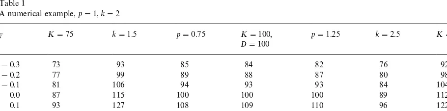
Table 1
A numerical example,p"1,k"2
c K"75 k"1.5 p"0.75 K"100, D"100
p"1.25 k"2.5 K"125
!0.3 73 93 85 84 82 76 92
!0.2 77 99 89 88 87 80 98
!0.1 81 106 94 93 93 84 104
0.0 87 115 100 100 100 89 112
0.1 93 127 108 109 110 96 122
0.2 102 148 118 121 123 102 138
0.3 116 197 136 142 148 118 167
Note:All numbers have been rounded o!to the nearest integer.
the process mean, or in this case the expected rate of in#ation. When in typical Bayesian fashion the prior density is revised as new (sample) information is received, the manager's posterior density will also be normal. Regardless of what that new informa-tion happens to be, the variance of the posterior density will always be given by pA2"p2/(n#n@), wherenis the number of sample observations [17, p. 128]. Therefore, the termp@2#p2in Eq. (4) can be replaced by
p2/(n#n@)#p2"p2[(n#n@#1)/(n#n@)Pp2
asnPR. As a consequence, when the manager's judgments as to the expected rate of in#ation are systematically revised as new data about the rate of in#ation are received, ceteris paribuscwill decline. The implication of this decline is that, ceteris paribus, we can anticipate that the optimum lot size will also decline over time.
The cross-partials with respect toK,k, andpare also readily computed and their signs readily deter-mined:
LM)N/LK"c/(e~cQ@D!1)(0, (7a) LM)N/Lk"(Q/2)[2#(Q/D)/(e~cQD!1)]'0, (7b) LM)N/Lp"D[1#(Q/D)/(e~cQD!1)]"$. (7c)
The sign ofcis the opposite of that of (e~cQ@D!1). Therefore,LM)N/LK(0 and hence dQH/dK'0. As
in the classic EOQ model, the optimum lot size increases when the set-up cost increases. Also as in the classic EOQ model, the optimum lot size decreases when the carrying cost increases.
This is so, since as previously determined,
D1#(cQ/D)/(e~cQD!1)D(1, which means that
LM)N/Lk'0, and therefore that dQH/dk(0. The
sign ofLM)N/Lp, however, will be the same as the
sign of 1#(cQ/D)/(e~cQD!1), and therefore it will be the opposite of the sign ofc. Hence, dQH/dpand
chave the same sign.
The latter result asserts the following. Suppose either the expected rate of in#ation exceeds the expected marginal cost of capital, or that there is su$cient uncertainty inherent in either the in#ation rate or the cost of capital so as to e!ectc'0. Then, the greater is the cost of acquiring the product to be inventoried, the greater will be the optimal lot size. When the expected rate of in#ation is su$ciently lower than the expected marginal cost of capital, so that even allowing for the uncertainty factor we get
c(0, then higher product-acquisition costs result in lower lot sizes. In essence, fears of in#ation or uncertainty about in#ation encourage greater pur-chases at `currenta prices. With a high marginal cost of capital and lower in#ation rates, however, uncertainty notwithstanding it will be preferable to tie up less capital than otherwise in acquiring inventory.
5. A numerical example
with varying values ofcin the [!0.3, 0.3] range, and for di!erent values ofp,k, andK, considered individually.
For ease of interpretation, all the optimal order quantities have been rounded o! to the nearest integer. The"gures may be veri"ed by substitution into Eq. (5). The numbers in the table are inter-preted as follows. In the central case, when
c"!0.3 the optimal order quantity decreases from its classicQH
c/0"100 level by 15% to 85. By
contrast, whenc"0.3, the optimal order quantity increases by 42% to 142. Whenp, say, increases to 1.25, the QHc/0"100 value is unaltered, but the other (rounded o!) optimal inventory levels decline or remain unchanged for c(0, and increase for
c'0. Precisely the reverse is true whenpdeclines to 0.75. That is, whenc"!0.2, for example, the optimal inventory increases from 88 to 89 when
pdeclines, but it decreases from 121 to 118 when
c"0.2. These results are what were foretold by the comparative statics implications of Eq. (7c). That is, when c(0, increases in the selling price result in decreased optimal lot sizes; and, when c'0, increases in the selling price result in increased optimal lot sizes.
Similarly, the results in the K and k columns were foretold by the comparative statics implica-tions of Eqs. (7a) and (7b). Regardless of the sign of
c, increases in the ordering cost increase the opti-mal lot size, and increases in the holding cost re-duce the optimal lot size.
In all instances it is apparent that QH is an increasing and strictly concave function ofc. In this regard, the example a$rms that although negative values forcwill not cause drastic deviations from
QH
c/0unless D!cD is fairly substantial, even quite
modest positive values ofccan wreak havoc with
QH
c/0. Thus, looking at Eq. (4), suppose that the
expected marginal cost of capital,R, is equal to the expected rate of in#ation,o. It is not hard to imag-ine circumstances under which the sum of the three variances in that equation would equal 0.4, say. Under those circumstances, c"0.2. Ignoring the uncertainty about the cost of capital and the rate of in#ation would result in settingQH
c/0"100, in the
central case, whereas taking those uncertainties into consideration results inQH
c/0.2"121. In this
example, then, ignoring the implications of
uncer-tainty results in a 17.4% understatement of the optimal lot size.
6. Conclusions
One of the few things upon which virtually all economists agree is that prices next year } any prices}are likely to be higher than are prices this year } any year. The only issue separating these economists is `how mucha higher, or what the future rate of in#ation will be. This is the case even though, for example, in recent years the United States as a case in point has enjoyed its lowest rates of in#ation in over a decade.
The pervasiveness and reality of in#ation is also recognized in operations management. For the past two decades the recognition has prompted at-tempts to incorporate in#ation into the analysis of inventory systems and to evaluate its impact upon optimal inventory policy in a dynamic and evolving world. The present paper continues that line of inquiry. The focus of that inquiry, however, is on how and whetheruncertaintyas to the rate of in# a-tion will impact upon optimal inventory policy in that world.
inventoried product will impact on the optimal lot size. Moreover, because all of these results are e! ec-ted through a discount factor ecthat is common to all extant dynamic inventory models that incorpor-ate the rincorpor-ate of in#ation, I would conjecture that the results are robust. It is, however, a conjecture that I leave to others to prove erroneous.
Appendix A
To establish the"rst-order condition for a min-imum, from Eq. (3@)
E[TC(Q)]"[KD/Q#pD#kQ/2][Q/D]
][(1!eac)/(1!ec(Q@D))].
Partially di!erentiating with respect toQwe obtain
LE[TC(Q)]/LQ"[(1!eac)/(1!ec(Q@D))][1/D]
]M[!KD/Q2#k/2]Q
#[KD/Q#pD#kQ/2]
#[KD/Q#pD#kQ/2][(cQ/D)
]ecQ@D/(1!ecQ@D)]N
"bM[!KD/Q#kQ/2]
#[KD/Q#pD#kQ/2]
][1#(cQ/D)/(e~cQD!1)]N.
Here,b'0, since (1!eac) and (1!ec(Q@D)) will be of the same sign for any value of c. Setting
LE[TC(Q)]/LQ"0 only requires that we set
M)N"0; or,
[!KD/Q2#k/2]Q#C 0[D/Q]
][1#(Q/D)ecQ@D/(1!ecQ@D)]"0. Eq. (5) immediately follows.
The second-order condition for a minimum is that
[LM[(1!eac)/(1!ec(Q@D))][1/D]N/LQ]M)N
#[LM)N/LQ][(1!eac)/(1!ec(Q@D))][1/D]'0.
But, M)N"0 from the "rst-order condition, and
[(1!eac)/(1!ec(QD))][1/D]'0. Therefore the sec-ond-order condition boils down toLM)N/LQ'0; or,
LM)N/LQ"[KD/Q2#k/2]#[!KD/Q2#k/2]
][1#(cQ/D)ecQ@D/(1!ecQ@D)]
#[KD/Q#pD#kQ/2]
]L[(cQ/D)ecQ@D/(1!ecQ@D)]LQ'0.
Now,
L[(cQ/D)ecQ@D/(1!ecQ@D)]LQ
"(c/D)[ecQ@D/(1!ecQ@D)][1#(cQ/D)/(1!ecQ@D)]. Gathering terms and for notational convenience again lettingy"cQ/D, the expression to the left of the inequality may be written as
k#[!KD/Q2#k/2][yey/(1!ey)]
#[KD/Q#pD#kQ/2](y/Q)[ey/(1!ey)]
][1#y/(1!ey)].
From the "rst-order condition, [!KD/Q2
#k/2]"!(C
0D/Q2)[1#yey/(1!ey)]. Making
this substitution into the previous equation and noting that [KD/Q#pD#kQ/2]"C
0(D/Q), the
equation may now be rewritten as
k!(C
0D/Q2)[1#yey/(1!ey)][yey/(1!ey)]
#(C
0D/Q2)[yey/(1!ey)][1#y/(1!ey)]
"k#(C
0D/Q2)[y2/(e~y!1)].
The latter expression is necessarily positive when
c(0, since in that case e~cQ@D'1. It is also easily veri"ed that the second-order condition holds for
c"0. The case ofc'0, however, is more complic-ated, since under those circumstances e~cQ@D!1(0. Forc'0, and once again taking advantage of the series expansion of e~cQ@D, we may write
c2/(e~cQ@D!1)
"c2/[!cQ/D][1!cQ/2D#c2Q2/6D2!2]. Therefore,
k#(C
0D/Q2)[y2/(e~y!1)]
"k!c[KD2/Q3#pD2/Q2#kD/Q]/ [1!cQ/2D#c2Q2/6D2!2].
When others have solved this and comparable problems for the case ofc'0, they have done so through some search procedure (see, e.g., [7]). As the present theoretical analysis would have pre-saged, the resulting solutions have indeed been large lot sizes, with the size increasing dramatically as the value ofc'0 increases.
References
[1] J.A. Buzacott, Economic order quantity with in#ation, Operational Research Quarterly 26 (3) (1975) 553}558. [2] H. Bierman Jr, J. Thomas, Inventory decisions under in#
a-tionary conditions, Decision Sciences 8 (1) (1977) 151}155. [3] R.B. Misra, A note on optimal inventory management under in#ation, Naval Research Logistics Quarterly 26 (2) (1979) 161}165.
[4] R.R. Jesse Jr, A. Mitra, J.F. Cox, EOQ formula: Is it valid under in#ationary conditions? Decision Sciences 14 (3) (1983) 370}374.
[5] J.M. Chandra, M.L. Bahner, The e!ects of in#ation and the value of money on some inventory systems, Interna-tional Journal of Production Research 23 (4) (1985) 723}730.
[6] T.K. Datta, A.K. Pal, E!ects of in#ation and time-value of money on an inventory model with linear time-dependent demand rate and shortages, European Journal of Opera-tional Research 52 (3) (1991) 326}333.
[7] B.R. Sarker, H. Pan, E!ects of in#ation and the time value of money on order quantity and allowable shortages, In-ternational Journal of Production Economics 34 (1) (1994) 65}72.
[8] M.A. Hariga, Economic analysis of dynamic inventory models with non-stationary costs and demand, Interna-tional Journal of Production Economics 36 (3) (1994) 255}266.
[9] M.A. Hariga, M. Ben-Daya, Optimal time varying lot-size models under in#ationary conditions, European Journal of Operational Research 89 (2) (1996) 313}325.
[10] J. Ray, K.S. Chaudhuri, An EOQ model with stock-depen-dent demand, shortage, in#ation and time discounting, International Journal of Production Economics 53 (2) (1997) 171}180.
[11] J.E. Golub, Does in#ation uncertainty increase with in# a-tion? Economic Review 79 (3) (1994) 27}38.
[12] A.S. Holland, In#ation and uncertainty: Tests for temporal ordering, Journal of Money, Credit, and Banking 27 (3) (1995) 827}837.
[13] G.K. Davis, B. Kanago, The missing link: Intra-country evidence on the relationship between high and uncertain in#ation from high-in#ation countries, Southern Eco-nomic Journal 63 (1) (1996) 205}225.
[14] Z.W. Kmietowicz, Y. Yannoulis, Statistical Tables for Eco-nomic, Business & Social Studies. Longman Scienti"c & Technical, Essex, 1988.
[15] J. Hirshleifer, On the theory of optimal investment deci-sion, Journal of Political Economy 66 (4) (1958) 329}352. [16] A. Je!rey, Handbook of Mathematical Formulas and
Inte-grals, Academic Press, London, 1995.
[17] J.O. Berger, Statistical Decision Theory and Bayesian Analysis, Springer, New York, 1985.
[18] W.K.K. Haneveld, R.H. Teunter, E!ects of discounting and demand rate variability on the EOQ, International Journal of Production Economics 54 (2) (1998) 173}192. [19] M. Hariga, M. Haouari, An EOQ lot sizing model with