Modelling the recent time trends in UK permanent health insurance
recovery, mortality and claim inception transition intensities
A.E. Renshaw, S. Haberman
∗Department of Actuarial Science and Statistics, City University, Northampton Square, London EC1V 0HB, UK
Received 1 March 1999; received in revised form 1 March 2000
Abstract
Models representing the underlying trends in UK permanent health insurance (PHI) recovery, mortality and claim inception transition intensitives over the 20 year calendar period, from 1975 to 1994 inclusive, are proposed. The investigation of such trends is of special interest given that the three transition intensities, with stationary estimates based on the equivalent grouped data for the quadrennial observation window 1975–1978, form an important part of UK continuous mortality investigation (CMI) Bureau multiple-state model for PHI business and play an important role in the pricing and reserving for PHI sickness benefits. © 2000 Elsevier Science B.V. All rights reserved.
Keywords:Permanent health insurance; Multi-state transition intensities; Trends
1. Introduction
The sickness recovery and inception transition intensities, together with the force of mortality when sick, which form the basis of UK continuous mortality investigation (CMI) Bureau’s multiple-state model, derive from the pooled experience of leading UK insurance companies in the observation window 1975–1978 (CMI, 1991). The introduction of this model (and the associated standard tables) represents a significant step forward in the ways in which the premiums and benefits for UK permanent health insurance (PHI) contracts could be valued, with implications for pricing and reserving, and in which the underlying transition experience could be measured and monitored. In this paper, our objective is to search for any significant underlying time trends (1975–1994) in these three fundamental transition intensities by “curve” fitting, noting that these trends might have important impli-cations for current practice in terms of the pricing and reserving for PHI sickness benefits. Sickness recovery intensities and mortality from sickness intensities are modelled, respectively, in Sections 2 and 3. As explained in Section 4, since there are added complications, which require further assumptions when modelling sickness
inception intensities as opposed to modelling the closely relatedclaiminception intensities, we model the latter. The implications of doing this are also discussed in Section 4. The investigation is made possible by the re-cent consolidation of the information provided by contributing offices to the PHI experience into a suitable data base.
∗Corresponding author. Tel.:+44-0171-477-8470; fax:+44-0171-477-8572. E-mail address:[email protected] (S. Haberman).
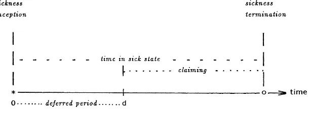
Fig. 1. Relationship between sickness inception and claim inception.
2. Sickness recovery intensities
2.1. Preliminaries
In this section, we model the sickness recovery transition intensities. Numbers of recoveries with matching exposures, in the raw data, have been made available by individual weeks for sickness duration, individual years for age at sickness inception and by individual calendar years, 1975–1994. This applies for each of five deferred periods of 1, 4, 13, 26, 52 weeks (DP1, DP4, DP13, DP26, DP52), for both males and females, see Fig. 1. Since the search for time trend patterns in the recovery intensities is a primary aim of the ensuing analysis, we have decided not to group the data by calendar year (typically grouped by quadrennia by the CMI Bureau for the purposes of monitoring the experience relative to the standard tables). There is ample exposure to permit this, without materially increasing the proportion of data cells void of exposure. For grouping with respect to both sickness duration and age at sickness inception, we follow the approach used in recent CMI Bureau commentaries on parts of the data set (see CMI, 1996), an arrangement which is judged to be satisfactory on the basis of trial and error. Hence, the complete cross-classification is summarised as follows:
gender male, female
deferred period 1, 4, 13, 26, 52 weeks
duration (z) 1–, 2–, 3–, 4–, 8–, 13–, 17–, 26–, 30–, 39–51 weeks, 1–, 2–, 5–11 years age (x) 18–, 25–, 30–, 35–, 40–, 45–, 50–, 55–, 60–64 years
period (t) 1975, 1976, 1977,. . ., 1994 (coded 1–20)
(Notationally, we follow CMI (1991) in usingzto indicate time and consequently usetto indicate years.) Note that there is a maximum of 13 duration levels subject to the specific deferred period, with 10 levels for DP4, eight levels for DP13, and so on. For each of the five deferred periods and each gender (10 separate cases), based on this cross-classification, let
rt xz= number of recoveries in cell (t,x,z)
et xz= exposure (in years) to the possibility of recovery in cell (t,x,z)
There is also a tendency for recoveries to be somewhat thinly spread across calendar years at sickness durations in excess of 2 years.
For a specific deferred period and specific gender, the recovery intensity per year from sicknessρt xzis targeted
by modelling the numbers of reported recoveries in the various data cells as Poisson response variables
rtxz∼Poi(etxzρtxz)independently for all cells(t, x, z)
for which
mtxz=E(rtxz)=etxzρtxz, Var(rtxz)=V (mtxz)=mtxz,
whereVis the variance function of the associated generalised linear model (GLM). (The scale parameter is one.) Hence the kernel of the log-likelihood is
Model fitting is implemented by optimising this expression using a log relationship
logmtxz=ηtxz=logetxz+logρtxz
linking the mean responsemt xzto a parameterised linear predictorηt xz. The second term logρt xzin the predictor
may be expressed as a variety of parameterised functions int,xandz, which are linear in the unknown parameters. Since the first term in the predictor loget xzdoes not involve any parameters, it is automatically subtracted from the
predictor in the fitting process and is described as an “offset” term. This means that this part of the predictor remains constant throughout the fitting of the different parameterised formulae forρt xz. Since each deferred period/gender
combination is modelled separately in this section, no notational provision for these two factors is required when formulating the model. The choice of a Poisson response GLM in this context is motivated by Sverdrup (1965). For a comprehensive discussion of GLMs, including applications, see McCullagh and Nelder (1989). For a review of actuarial applications of GLMs, see Haberman and Renshaw (1996).
2.2. Male, DP1 experience
2.2.1. Model selection
Following exploratory analysis, centred mainly on investigating the relative merits of using low order poly-nomial structures in√z, as opposed toz, for individual calendar years, we take as our starting point the model structure
logρxz=β0+β1√z+β2z+β3x+β4x√z+β5xz,
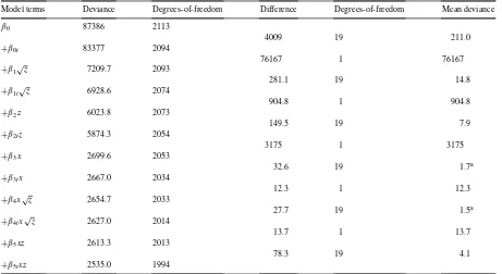
Table 1
Deviance profile, Eq. (2.1): male, DP1 experience
Model terms Deviance Degrees-of-freedom Difference Degrees-of-freedom Mean deviance
β0 87386 2113
It is possible to assess the significance of the various sets of parameters by fitting these sequentially and conducting an analysis of deviance. One such possibility based on the order in which the terms appear on the RHS of Eq. (2.1), is reported in Table 1. Firstly, note that the order in which the parameters were fitted, may be deduced by reading down the first column. Then, for a Poisson GLM, as here, the model deviances reported in the second column of the table, are given by (e.g. McCullagh and Nelder, 1989, p. 34)
X
wheremˆtxzdenote the predicted number of recoveries (fitted values) under the specific predictor structure anddt xz
is the contribution to the model deviance from the data cell defined by (t,x,z), with weightωtxz=0 if a data cell has zero exposure, and weightωtxz =1, otherwise. The number of degrees-of-freedom reported in the third column, is equal to the sum of these weights (the number of non-empty cells) minus the number of effective parameters included in the linear predictor structure. Columns 4 and 5 of Table 1 are constructed by differencing the respective model deviances and matching degrees-of-freedom and the mean deviance (based on the ratios of these differences) are recorded in the last column. The entries in the last three columns of Table 1 monitor the significance of the parameter(s) identified by the matching adjacent (lower) entry in the first column. Then, under the assumption that the difference in the deviances (column 4) are approximately distributed asχ2(exact in the case of Gaussian response GLMs), we set the parameters{β3t}and{β4t}equal to zero on the basis that they are not statistically
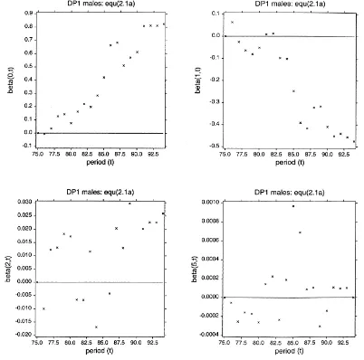
Fig. 2. Parameter plots: Eq. (2.1a).
involving an analysis of deviance relating to car insurance claims and which is similar to the present case, albeit based on a gamma response GLM, see Section 8.4.1 of McCullagh and Nelder (1989).
We, therefore, fit the simplified model structure
logρtxz=(β0+β0t)+(β1+β1t)√z+(β2+β2t)z+β3x+β4x√z+(β5+β5t)xz (2.1a)
and search for possible time trends by plotting each of the resulting sets of parameter estimates{ ˆβ0t},{ ˆβ1t},{ ˆβ2t}
and{ ˆβ5t}against timet. These plots are reproduced in Fig. 2. Focusing first on the bottom right hand frame which
relates to{β5t}, on the basis of this visual evidence that the plotted points are not supportive of any trend; coupled
with the information that only two out of the 19 parameters differ significantly from zero (established by individual
t-statistics), we have decided to further simplify the model by also setting the parameters{β5t}equal to zero. We note
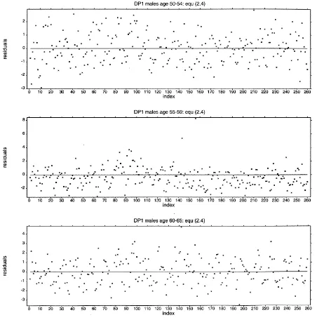
Fig. 3. Residual plots: Eq. (2.4).
cell (t =1986,x =55–59,z=5–11 years) corresponds to the extreme case of two acknowledged poor quality data cells involving sickness duration 5–11 years. We have decided to retain such data cells and note their appearance as outliers in the ensuing residual plots (e.g. Fig. 3). Secondly, on the basis of the three remaining estimator plots of Fig. 2, which exhibit straight line trends (with relatively little dispersion in two cases), we have decided to trade some local variation (within the context of the heavily parameterised model (2.1a)), for the nine parameter model
Table 2
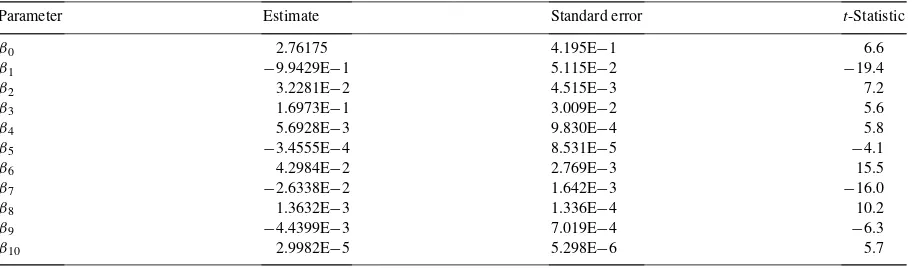
Parameter estimates, standard errors,t-statistics, Eq. (2.4): male, DP1 experience
Parameter Estimate Standard error t-Statistic
Finally, noting that the RHS of Eq. (2.3) is now a polynomial in the three variatest,xand√z, we experiment by introducing additional polynomial terms in the threevariates, using as a criterion a significant reduction in the model deviancecoupledwith the retention of a complete set of statistically significant parameter estimates. On this basis, Eq. (2.3) is modified to include additional parameterised terms inx2andx3, a feature which induces a further reduction of 110.4 in the deviance for the loss of 2 degrees-of-freedom. This leads finally to the adoption of the model structure
logρtxz=β0+β1√z+β2z+β3x+β4x√z+β5xz+β6t+β7t√z+β8tz+β9x2+β10x3. (2.4) The parameter estimates, together with their standard errors and t-statistics, are presented in Table 2. Separate investigations (not reported here) demonstrate the credibility of this model structure. For example, grouping the data by four year calendar periods, it transpires that, for each of 1975–1978, 1979–1982,. . ., 1991–1994, a model of the type (2.4), with the time dependent parameters (β6,β7,β8) pre-set to zero, provides a satisfactory fit to the recovery transition intensities (for males for deferred period equal to 1 week).
2.2.2. Model interpretation
Diagnostic checks of the model structure are conducted using deviance residuals, defined by
sign(rtxz− ˆmtxz)ωtxz
p
dtxz,
wheredt xzare the components of the model deviance, defined in Eq. (2.2). A variety of residual plots have been
examined. For example, deviance residuals plotted against the index (or counter)
index(t, z′)=z′+z∗(t−1)
based on durationcategoriesz′ =1,2, . . . , z∗ (z∗ =13 for DP1,z∗ =10 for DP4, etc.) serialised by calendar
yeart = 1,2, . . . ,20, for each separate age category, provides a compact way of viewing the residuals plotted
against sickness duration, arranged end-on for each period. Thus, for a specified age, the firstz∗points on the index represent the full range of possible sickness durations, arranged in increasing order, for 1975, then for 1976, and so on. By way of illustration we reproduce three such plots in Fig. 3. Note in particular the outlier described earlier, together with a further outlier.
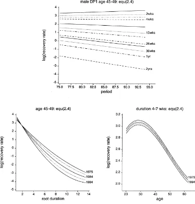
The structured model (2.4) may be interpreted as a three-dimensional surface int,xand√z(for values ofzless than 5 years so as to avoid durations where the data are particularly sparse). This model may be viewed from a number perspectives, which include the following:
Perspective1:
where
Perspective 1 focuses on the model prediction that, for fixed (x,z), the log-recovery intensity has changed linearly in time over the 20 year calendar period. Note that the behaviour of the signs ofBxzover the (x,z) grid is of special
interest, since these dictate the cells for which the predicted recovery intensities have increased or decreased over the period concerned. On noting thatBxzis independent ofxand is a quadratic in√z(c.f. a(√z)2+b√z+c,
with negativeaand positive discriminantb2−4ac>0, see Table 2 for parameter values), it follows thatBxzis
positive, and hence the predicted recovery intensities decrease, for values of√zbetween the roots 1.80 and 17.52 of the quadratic. In essence, these imply that recovery intensities have increased over time for sickness durations of 3 weeks and under and for durations 307 weeks and over, but otherwise have been in decline during the period of investigation. We return to the quadratic form forBxz in Section 2.6. Predicted log-recovery intensities, plotted
against calendar period, for specific ages at sickness inception are reproduced in the upper frame of Fig. 4. Perspective 2 focuses on the log-recovery intensity, viewed as a function of sickness duration, for fixed (t,x). It is a quadratic in√z, withCt x, the coefficient of(√z)2, positive for all values of (t,x) within the domain defined by
the data grid. Hence, the quadratic is convex, with a turning point that is a minimum. A typical family of quadratics for eacht, fixedx, is illustrated in the bottom left frame of Fig. 4, in which the turning point lies “off the chosen scale”.
Perspective 3 focuses on the prediction that log-recovery intensities change as a cubic function in agex. This feature is illustrated in the bottom right frame of Fig. 4, in which a typical family of cubic profiles, for different calendar periods and specific policy duration, is presented. Note that calendar period effects impact only on the coefficientAt z, thereby inducing parallel cubic curves. Further, over the relevant age range, 18–65 years, it can be
shown that the cubic expression inxhas a maximum at age
49.36−1.96
q
(√z−8.24)2+75.20
with a point of inflexion at age 49.36.
2.3. Male, other deferred periods
2.3.1. Model selection
A different model is needed for each of the other deferred periods. We take as our starting point the model structure
Fig. 4. Log-recovery rates vs. various perspectives: Eq. (2.4).
where(z−zj)+ =z−zjifz > zj, and(z−zj)+ =0 ifz≤zj. This has been fitted previously (Renshaw and
Haberman, 1995), to versions of the grouped 1975–1978 quadrennium data sets for DP4, DP13 and DP26. We again begin by fitting the structure separately for each calendar year, so that
logρtxz =(β0+β0t)+(β1+β1t)x+(β2+β2t)z+(β3+β3t)(z−z0)+
+(β4+β4t)(z−z1)++(β5+β5t)x(z−z0)+ (2.5)
subject to the constraints
β01 =β11=β21 =β31=β41 =β51=0.
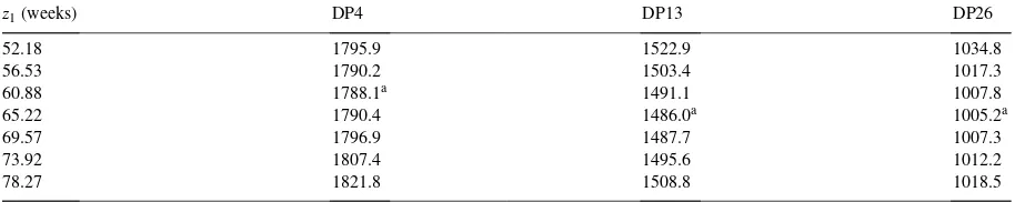
Table 3
Deviance profiles for knot settings, Eq. (2.5): male experiences
z1(weeks) DP4 DP13 DP26
Table 4 (Continued)
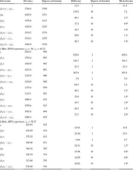
Model terms Deviance Degrees-of-freedom Difference Degrees-of-freedom Mean deviance
rates in the first 4 weeks immediately after sickness benefit becomes payable, for the male experience for the 1975–1978 quadrennium. This feature has been further investigated and found to persist throughout the 20 year period under investigation. The details are available from the authors on request. In addition, it may be further assessed by referring to the degree of statistical significance associated with the parameters β3 andβ5 in the ensuing analysis.
The separate analysis for DP4, DP13 and DP26 follows a near identical pattern, subject to decreasing overall exposure with increasing (fixed) deferred period. Firstly, the optimum position of the second knotz1is determined by the repeated fitting of model structure (2.5), under incremental changes of 1 month (based on a 12 month year, each of length 4.35 weeks) in the position ofz1. The resulting deviance profiles are reported in Table 3, and the optimum value ofz1is selected accordingly.
For DP52, it is necessary to pre-setβ3 = β3t = β5 = β5t =0 since the associated data are not amenable to
the specific investigation of the 4 week “run-in” period. Neither are these data amenable to the construction of a finely graded deviance profile as above, due to the necessary broad grouping of the raw data. Consequently, we have set the knot at the centre of the first sickness band. Next, the deviance profiles, as the terms on the RHS of Eq. (2.5) are added sequentially into the structure of the model, are reported in Table 4 (a)–(d). Here, as implied by the first column of each of these tables, we have introduced all the parameters which do not display period effects in the first instance, and then added in the parameters representing the period effects. On the basis of the statistical significance, or otherwise, of the deviance differences (column 4) when referred to an approximateχ2distribution, the conclusions are similar in all four cases, leading to the adoption of the simplified model structure
logρtxz=β0+β0t +β1x+β2z+β3(z−z0)++β4(z−z1)++β5x(z−z0)+ (2.5a)
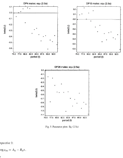
for DP4, DP13, DP26, and with additionallyβ0t =0(β3 =β5 =0)for DP52. Finally, since the ensuing{β0t}
time patterns, reproduced in Fig. 5, exhibit essentially straight line trends, we trade some local variation, within the context of the model (2.5a), by settingβ0t =α+β6t(and absorbing the parameterαintoβ0) and adopt the model structure
logρtxz=β0+β1x+β2z+β3(z−z0)++β4(z−z1)++β5x(z−z0)++β6t (2.6) for DP4, DP13, DP26 with additionallyβ3=β5=β6=0 for DP52.
2.3.2. Model interpretation
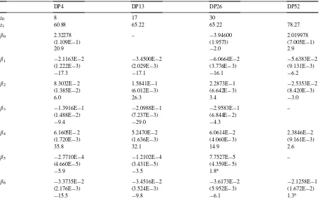
The parameter estimates, together with their standard errors andt-statistics, for all four cases, are presented in Table 5. Note that we have retained the period effects out of interest in the case of DP52, in spite of the fact that they are not statistically significant, a feature confirmed by the value of thet-statistic of the relevant parameter. Diagnostic checks are again based on deviance residual plots, typical examples of which are reproduced in Fig. 6.
Eq. (2.6) may be viewed from the same three perspectives as Eq. (2.4), namely
Fig. 5. Parameter plots: Eq. (2.5a).
Perspective3:
logρtxz=Atz−Btzx,
where
Atz=β0+β2z+β3(z−z0)++β4(z−z1)++β6t, Btz= −β1−β5(z−z0)+.
Under Perspective 1,Bxz is positive for all four deferred periods, so that the predicted log-recovery intensities
Table 5
Parameter estimates, standard errors,t-statistics, Eq. (2.6): males
DP4 DP13 DP26 DP52
of the three line segments for each of DP4, DP13, DP26 are given by
Btx=β2, z≤DP+4, Btx+Ctx=β2+β3+β5x, DP+4< z≤z1,
Btx+Ctx+Dtx=β2+β3+β4+β5x, z > z1.
It then follows trivially from Table 5 that the predicted log-recovery intensities first increase in the so-called 4 week “run-in” durational period, then decrease linearly with increasing sickness duration, for fixed (t,x), and generally continue to decrease but less rapidly so for durations in excess ofz1weeks. The lower frame in Fig. 7 illustrates this. Under Perspective 3,Btz >0 and the predicted log-recovery intensities decrease linearly with age at sickness inception, for fixed (t,z).
2.4. Female, DP1 experience
In the absence of any reported previous analysis of UK female PHI experience (e.g. from the 1975–1978 investi-gation), we follow the same approach as that adopted in Section 2.2 for the male experience, while noting that the female experience is much more sparse than the corresponding male experience. The deviance profile associated with the sequential fitting of the terms on the RHS of expression (2.1) is reported in Table 6. While the approximate
Fig. 6. Residual plots (DP13): Eq. (2.6).
the experience is not supportive of any statistically significant period effects in the sets of parameters with the possible exception of the{β0t}. The parameter estimates{ ˆβ0t}under the fitted model structure
logρtxz=(β0+β0t)+β1√z+β2z+β3x+β4x√z+β5xz
Fig. 7. Log-recovery rates vs. various perspectives: Eq. (2.6).
obvious time trend. This is further supported by fitting the model structure
logρtxz=β0+β1√z+β2z+β3x+β4x√z+β5xz+β6t (2.7) in which we have setβ0t =α+β6tin the foregoing equation and replacedβ0+αbyβ0. Eq. (2.7) can, in turn, be rewritten as
Perspective1:
logρtxz=Axz−Bxzt,
where
Table 6
Deviance profile, Eq. (2.1): female, DP1 experience
Model terms Deviance Degrees-of-freedom Difference Degrees-of-freedom Mean deviance
β0 9239.4 1684
The parameter estimates, standard errors, andt-statistics are reported in Table 7. These indicate that the period effect is not statistically significant, but that, sinceBxz <0, there is some weak evidence to support the general statement that recovery intensities have increased, if anything, over the 20 year period concerned. The quality of the fit has again been assessed by the residual plots associated with the fitted structure, two of which are reproduced in the lower frames of Fig. 8.
2.5. Female, other deferred periods
Structure (2.6), fitted to the equivalent male experiences in Section 2.3, has also been fitted to the female DP4, DP13 and DP26 experience but withβ5pre-set to zero, as the product termx(z−z0)+proved to be statistically
non-significant in this case. The optimum position of the knot in each case, is determined by reference to deviance
Table 7
Parameter estimates, standard errors,t-statistics, Eq. (2.7): female, DP1 experience
Fig. 8. Parameters plot: Eq. (2.5a) and residual plots: Eq. (2.7).
profiles (as in Section 2.3), constructed by varying the position of the knot by monthly increments in the model (2.6), the results of which are reported in Table 8. We can again write the model structure as
Perspective1:
logρtxz=Axz−Bxzt,
where
Table 8
Deviance profiles for knot settings, Eq. (2.6): female experiences
z1(weeks) DP4 DP13 DP26
Parameter estimates, standard errors,t-statistics, Eq. (2.5): females
DP4 DP13 DP26
in order to highlight the dependence ont. Details of the parameter estimates are reported in Table 9. Additionally, we have pre-set β0 to zero for DP13 since, in the event, this term also proves to be statistically insignificant. Since the estimated value of β6 is negative for each deferred period, there is an implied deterioration in the recovery rates over the 20 year period concerned. Perspectives 2 and 3 are similar in outline to the equivalent male experiences.
2.6. Discussion of results
It is of interest to compare the magnitudes ofBxz, the rates by which the predicted log-recovery intensities change
(x,z). Consequently, it is a simple matter to compare rates in these cases by tabulating the values of−Bxz =β6, say, taken from Tables 5, 7 and 9. Thus
DP1 DP4 DP13 DP26 DP52
with anegativesign implying decreasing recovery intensities over time. The similarity of the results for the male DP4, DP13 and DP26 experience, together with the female DP13, DP26 experience, and to a lesser extent the female DP4 experience, is noteworthy. The situation is somewhat more complex for the male DP1 experience, withBxz dependent onz. For this experience, recovery intensities decrease with time for durations in excess of 4
weeks but less than 6 years. Discussions with reinsurers and direct insurers active in the PHI market in UK suggest that a possible explanation for the increase in recovery rates with time at these short sickness durations for DP1 policies could be the improved management of claims by insurers over this period, together with a move to active intervention in newly admitted claims. These changes may have led to fewer marginal cases being accepted as new claims; to accepted claims being managed more actively at the short durations, leading to increased short duration recoveries; and to the residual claims, surviving this initial, active management stage, being the more problematic and long term cases. These effects would be particularly noticeable for shorter deferred policies, as these would provide greater scope for early intervention in any newly notified claims. For longer deferred period policies, claims would be notified somewhat later and tend to be more established by the time that the insurer’s claims management process could intervene. These changes could explain the difference in the nature of the results for DP1 compared to the longer deferred periods.
3. Mortality from sickness intensities
In this section, we focus on the force of mortality when in the sick state. Because of the relatively low reported incidence of sick to death transitions, in keeping with previous work by the CMI Bureau on such transitions (Section 5, Part B of CMI (1991)), the deaths and exposures in matching cells are combined by summation over all deferred periods (DP1, DP4, DP13, DP26, DP52), and the cross-classified data cells are defined by
gender (g) 1 — male, 2 — female
duration (z) 1–, 4–, 8–, 13–, 17–, 26–, 30–, 39–51 weeks, 1–, 2–, 5–11 years (11 levels) age (x) 18–, 35–, 40–, 45–, 50–, 55–, 60–64 years (7 levels)
period (t) 1975–1978, 1979–1982, 1983–1986, 1987–1990, 1991–1994 (5 quadrennia)
with calendar years grouped as quadrennia, unlike Section 2. Hence the raw data used in this analysis comprise
dtxzg number of deaths in sick cell (g,t,x,z)
egtxzexposure (in years) to risk of death in sick cell (g,t,x,z)
The force of mortality when sick (or mortality from sickness transition intensity)νtxzg is targeted by assuming that the numbers of reported deaths in the various data cells to be independent Poisson response variables
dtxzg ∼Poi(egtxzνtxzg )independently for all cells(g, t, x, z)
for which
Table 10
Deviance profile, Eq. (3.1)
Model term Deviance Degrees-of-freedom Difference Degrees-of-freedom Mean deviance
µ 1618.3 763
whereVis the variance function of the associated GLM. (The scale parameter is one.) This assumption forms the basis of recent approaches to the actuarial graduation of the force of mortality for assured lives, annuitants and pensioners (Forfar et al., 1988; Renshaw, 1991). It can also be justified on the basis of Sverdrup (1965), as noted in Section 2.1. Model fitting is implemented in combination with the log-link predictor relationship
ηgtxz=logmgtxz=logegtxz+logνtxzg ,
whereηgtxzdenotes the linear predictor, logegtxzthe offset and logνtxzg is expressible as a variety of parameterised functions in the four covariates, gender, period, age and sickness duration. Note that, unlike Section 2, we model gender as a covariate since there are insufficient data to model the female experience separately. An exploratory analysis is possible by modelling all four covariates as categorical factors. In particular, the main effects structure takes the parametric form
logνgtxz=µ+αg+βt+γx+δz. (3.1)
It is of interest to note that this is an extension, involving additional calendar period and gender effects, of the multiplicative structure (under the inverse log-link) investigated by Bayliss (1991) in relation to the 1975–1978 male experience, and which was identified as a Poisson GLM with a log-link by Renshaw and Haberman (1995).
One of the possible ways in which the factors can be added sequentially into the structure of the RHS of Eq. (3.1) is recorded in Table 10. Again, the order of the sequencing may be deduced by reading down the first column of the table, and, on the basis that the deviance differences are approximately distributed asχ2, all four factors are established as being highly significant statistically.
The feasibility of incorporating additional paired interactions terms into the predictor structure was subsequently investigated and quickly abandoned, owing to the paucity of recorded deaths from sick in many of the cross-classified data cells, especially for females. Indeed the total number of recorded female deaths across all cells making up the five quadrennia are as follows:
1975–1978 1979–1982 1983–1986 1987–1990 1990–1994
19 19 28 41 58
Deviance residual plots generated by the main effects model structure (3.1) are presented in Fig. 9. These comprise plots of the residuals against an age/duration index, separately for males in each of the five quadrennia, and for all females combined over all 20 calendar years. The index is defined as
Fig. 9. Residual plots: Eq. (3.1).
wherezi, with values 1–11, identify the 11 duration groups arranged in increasing order; and similarly xi, with
values 1–7, identify the seven age groups arranged in increasing order. It is arranged, so that thez’s are nested within thex’s. Thus, the first 11 points on the index represent the full range of possible sickness durations, arranged in increasing order of magnitude, for ages 18–34, etc.
The parameter estimates for the main effects structure, Eq. (3.1), make interesting reading. The details are presented in Table 11. The model predicts that mortality rates from the sick state:
Table 11
Parameter estimates, standard errors,t-statistics, Eq. (3.1)a
Parameter Estimate Standard error t-Statistic
3. improve progressively over the five quadrennial calendar periods,
4. are essentially bell-shaped with respect to sickness duration, deteriorating up to duration 26–29 weeks, followed by a relative improvement as duration further increases, with an apparent final up-turn in mortality at very long durations.
These effects are graphically illustrated in the upper frame of Fig. 10, in which the predicted log-mortality intensity logνtxzg , is plotted against duration (on the categorical scalezi), for each age bandxi, for the 1975–1978
male experience (withβ1 =0, αg =0: note that the first level of each batch of parameters is set equal to zero,
by convention within the GLIM modelling computer system on account of over-parameterisation in the model structure). We recall that the 1975–1978 male experience formed the basis for the construction of the PHI standard model in current use in UK. It is of interest to note that the general shape of the graphs in the upper frame of Fig. 10 is consistent with the so-called duration factor profile, Figure B6 of Bayliss (1991), based on that author’s analysis of the 1975–1978 male experience. In addition, the age factor profile in Figure B7 of Bayliss (1991) is consistent with the pattern in the age effects parameter estimatesγˆxof Table 11, with again statistically insignificant
effects for ages under 40 years, as implied for the 1975–1978 experience of Bayliss (1991, p. 36). The parallel profile, representing each of the age bands in Fig. 10, is a feature of the additive, non-interactive, nature of the linear predictor structure. Identical profiles, constructed by moving (loweringsince both the estimatedαg’s and the
estimatedβt’s are negative) the whole configuration vertically relative to the ordinate by an amountαg+βt, apply
for the nine remaining period/gender combinations under study. These profiles imply a reduction in mortality for each age/duration cell relative to the 1975–1978 male experience. It is also of interest to note, that while the CMI (1991) model is based onνtxzg depending onx(attained age) only, for sickness duration sickness durationzin excess of 5 years, it follows from Table 11 that the parameter estimates for durational main effects,δˆz, are of borderline
Fig. 10. Log-mortality rates: Eqs. (3.1) and (3.2).
Given the patterns in the sets of parameter estimates (Table 11), it is further possible to reduce the number of parameters utilised by representing all three of the covariates — period, age and duration — as continuous variates and incorporating them into the formula
logνgtxz=β0+αg+β1x+β2z+
k
X
j=1
βj+2(z−zj)++βk+3t, (3.2)
where
α1=0 for males, (z−zj)+=
(
z−zj, z > zj,
Table 12
Parameter estimates, standard errors,t-statistics, Eq. (3.2)a
Parameter Estimate Standard error t-Statistic
Here, periodtis coded from 1 to 5 (to match the respective quadrennia), while agex(in years) andz(in weeks) are allocated values at the centres of the relevant data cells defined at the outset of this section. In Eq. (3.2), duration effects are represented by hinged line segments, withkhinges or knots positioned atzjε{2.5, 6, 10.5, 15, 21.5, 28,
34.6, 45.6, 78.3, 182.6, 417.4}. A similar structure withα2=β5=0, k=2, was fitted to an earlier version of the 1975–1978 males experience, Renshaw and Haberman (1995). To accord with the basic shape of the upper frame in Fig. 10 we elect to site four knots atz1=10.5, z2=28, z3=45.6, z4=182.6, corresponding to the key changes in direction. Details of the fit, in which all parameters estimates are shown to be highly significant statistically, are reported in Table 12. The resulting predicted log-mortality intensity is plotted against duration, now measured in weeks, for each age, for the 1975–1978 male experience (t=1,αg =0) in the lower frame of Fig. 10. The overall
patterns in the corresponding residuals are similar in nature to those associated with model (3.1), as reported in Fig. 9, and are hence not reproduced. The conclusions to be drawn from model (3.2) are similar to those drawn from model (3.1), i.e. (1)–(4) as presented above.
4. Claim inception intensities
4.1. Preliminaries
In this section, we report on the claim inception intensities. The raw data comprise claim inception counts with matching exposures, cross-classified according to the format
gender male, female
deferred period 1, 4, 13, 26, 52 weeks
age at inception (x) 18–, 25–, 30–, 35–, 40–, 45–, 50–, 55–, 60–64 years calendar time at inception (t) 1975, 1976, 1977,. . ., 1994
For each gender in combination with each of the five deferred periods, let
it x claim inception count in cell (t,x)
et x matching exposure in cell (t,x)
as the case may be. Thus,it xrepresents the number of sicknesses which start in the observation cell (t,x) and which
The claim inception transition intensity τt x is targeted for specific gender and deferred period combinations.
This is done by declaring the numbers of reported incidents of claims in the various data cells to be independent over-dispersed Poisson response variables, such that
mtx=E(itx)=etxτtx, Var(itx)=φ V (mtx)=φmtx
with variance functionV, and scale parameterφ. The scale parameter is included in recognition of the presence of duplicates amongst the policies contributing to the data base. Such responses are implemented in combination with the log-link predictor relationship
ηtx=logmtx=logetx+logτtx,
whereηt xdenotes the linear predictor and loget xthe offset.
It is informative to relate the targeting of claim inception transitionsτt x to that of targeting sickness inception
transitionsσt x, since the latter play a more fundamental role in the PHI multiple-state model. The claim and sickness
inception intensities are related byτtx=πtxdσtx, whereπt xd denotes the probability that the time spent in the sick
state exceeds the relevant deferred period ofd(=1, 4, 13, 26, 52) weeks. Hence, when targetingσt xas opposed to
τt x, it would first be necessary to determine values forπt xd, so that logπt xdmay be added to the offset term prior
to model fitting. It is possible to do this by evaluating the integral
πtxω =exp
However, the resulting predicted sickness inceptions are sensitive to the values ofπt xd, a feature noted in Renshaw
and Haberman (1995), and we have elected to model and report on trends in the claim inception rates which we believe are also of great interest to practitioners, in particular, for the measurement and monitoring of emerging claims experience. Others have followed this route of attempting to model directly the claim inception rates: see, e.g. Dillner (1969) and Haberman and Walsh (1998). The modelling of the sickness inception transitionsσt xcoupled
with the evaluation ofπt xωis being investigated further.
For each separate DP (and gender), focus on model structures of the type (as suggested by Renshaw et al. (1996) in the context of mortality)
in which both agexand calendar yeartat sickness inception are modelled as continuous variates. Specifically,xis allocated values at the centre of the relevant age cell (as defined above), whilet(as defined above) is mapped into
t′usingt′= 91.5(t−1984.5), so thatt′takes one of 20 equally spaced values in the interval [−1, 1] corresponding to the calendar years 1975–1994 inclusive. There are potential computational advantages in usingt′ rather thant. Where the results dictate that certain of the parameters in Eq. (4.1) are not statistically significant, they are pre-set to zero.
4.2. Male experiences
Specific details of the model structures (4.1) fitted separately for each DP may be deduced from Table 13 which tabulates the relevant parameter estimates, their standard errors and “t-statistics”. The nature of these predictor structures is summarised thus
DP1 quintic inteffects+cubic inxeffects+second and third order product effects DP4 quintic inteffects+cubic inxeffects+second order product effects
Table 13
Parameter estimates, standard errors,t-statistics, Eq. (4.1): male experience
DP1 DP4 DP13 DP26 DP52
Standard error 8.659E−2 1.571E−1
t-Statistic −3.9 −3.7
α5 1.5696 6.9474E−1 – – –
Standard error 1.992E−1 3.038E−1
t-Statistic 7.9 2.3
DP26 cubic inteffects+cubic inxeffects
DP52 linear inteffects+cubic inxeffects+second order product effects.
Table 14
Parameter estimates, standard errors,t-statistics, Eq. (4.1): female experience
DP1 DP4 DP13 DP26
Standard error 1.913E−4 2.553E−4
t-Statistic −6.7 −3.7
γ11 2.2616E−2 1.3073E−2 – –
Standard error 3.655E−3 5.119E−3
t-Statistic 6.2 2.6
ˆ
φ 2.343 1.463 1.256 1.487
(1998) analysis of claim inception intensity trends over the shorter time period 1987–1994 led to unconvincing results, which were encapsulated in a model that was “quadratic inteffects and quinticxeffects” with no product terms.
Each structure has been selected on the basis of exploratory data analysis involving an examination of deviance profiles, deviance residual plots and the statistical significance or otherwise of the associated parameter estimates. In particular, residuals plotted against both age and calendar year of sickness inception are especially informative. Given the presence of a free standing scale parameterφ in this analysis, here we make use of scaled deviance residuals
By way of illustration we reproduce three such plots in Fig. 11.
The resulting smoothed log-claim inception intensities generated by these models for DP1, DP4, DP13 and DP26 are illustrated in Fig. 12, with each figure comprising separate plots of the predicted log-claim inception intensities against calendar year for each age. The cyclical appearance of these curves leads to the suggestion of an association with indices of the economic cycle, and a possible causal link: this is a potential area for further work: see Section 5 (and the preliminary analysis of Haberman and Walsh (1998)).
4.3. Female experiences
Similarly, Table 14 presents specific details of the model structures (4.1) fitted separately for each DP (except DP52). The nature of the predictor structures is summarised thus:
Fig. 11. Residual plots: Eq. (4.1).
DP4 linear inteffects+quadratic inxeffects+second order product effects DP13 linear inxeffects
DP26 linear inteffects+linear inxeffects DP52 paucity of data
Fig. 12. Log-claim inception intensities: Eq. (4.1).
5. Further work
We have identified a number of areas worthy of further investigation:
Fig. 13. Log-claim inception intensities: Eq. (4.1).
2. Consideration of the recoveries split into broad categories by type of disability in order to investigate the hypothesis that certain types would be more susceptible to economic trends. This would be dependent on the relevant data being provided by the CMI Bureau.
Acknowledgements
The authors wish to thank the CMI Bureau for providing both financial support and the data, and in particular for generously giving of its time to respond to various queries concerning the data. The authors would also like to thank David Heeney, Mark Hills and Duncan Walsh, together with an unknown referee, for helpful comments on earlier drafts.
References
Bayliss, P.H., 1991. The graduation of claim recovery and mortality intensities. CMIR 12, 21–50.
CMI Committee, 1991. The analysis of permanent health insurance data. Continuous Mortality Investigation Report No. 12. Institute of Actuaries. CMI Committee, 1996. Recovery rates under PHI policies, individually 1975–90 and grouped 1975–86. Continuous Mortality Investigation
Report No. 15. Institute of Actuaries, pp. 1–50.
Dillner, C.G., 1969. New bases for non-cancellable sickness insurance in Sweden. Skandinavisk Aktuarietidskrift 52, 113–124. Forfar, D.O., McCutcheon, J.J., Wilkie, A.D., 1988. On graduation by mathematical formula. J. Inst. Actuaries 115, 1–149. Haberman, S., Renshaw, A.E., 1996. Generalised linear models and actuarial science. J. R. Statist. Soc., Ser. D 45, 407–436. Haberman, S., Walsh, D.J.P., 1998. Analysis of trends in PHI claim inceptions data. Trans. 26th Int. Congress Actuaries 6, 159–186. McCullagh, P., Nelder, J.A., 1989. Generalised Linear Models. Chapman & Hall, London.
McNown, R., Roberts, A., 1989. Forecasting mortality: a parameterised time series approach. Demography 26, 645–660. Renshaw, A.E., 1991. Actuarial graduation practice and generalised linear and non-linear models. J. Inst. Actuaries 118, 295–312.
Renshaw, A.E., Haberman, S., 1995. On the graduations associated with a multiple state model for permanent health insurance. Insurance: Mathematics and Economics 17, 1–17.
Renshaw, A.E., Haberman, S., Hatzopolous, P., 1996. The modelling of recent mortality trends in UK male assured lives. Br. Actuarial J. 2, 449–477.