Full Terms & Conditions of access and use can be found at
http://www.tandfonline.com/action/journalInformation?journalCode=ubes20
Download by: [Universitas Maritim Raja Ali Haji] Date: 12 January 2016, At: 17:18
Journal of Business & Economic Statistics
ISSN: 0735-0015 (Print) 1537-2707 (Online) Journal homepage: http://www.tandfonline.com/loi/ubes20
A Penalty Function Approach to Bias Reduction in
Nonlinear Panel Models with Fixed Effects
C. Alan Bester & Christian Hansen
To cite this article: C. Alan Bester & Christian Hansen (2009) A Penalty Function Approach to
Bias Reduction in Nonlinear Panel Models with Fixed Effects, Journal of Business & Economic Statistics, 27:2, 131-148, DOI: 10.1198/jbes.2009.0012
To link to this article: http://dx.doi.org/10.1198/jbes.2009.0012
Published online: 01 Jan 2012.
Submit your article to this journal
Article views: 411
View related articles
A Penalty Function Approach to Bias Reduction
in Nonlinear Panel Models with Fixed Effects
C. Alan BESTER
University of Chicago, Graduate School of Business, Chicago, IL 60637 (cbester@chicagosb.edu)
Christian HANSEN
University of Chicago, Graduate School of Business, Chicago, IL 60637 (chansen1@chicagosb.edu)
We consider estimation of nonlinear panel data models with individual specific fixed effects. Estimation of these models is complicated since estimation of the fixed effects when the time dimension is short generally results in inconsistent estimates of all model parameters. We present a penalized objective function that reduces the bias in the resulting point estimates. The penalty function is simple to construct and requires no modification for models with multiple individual specific parameters. We illustrate the approach through a series of simulations that suggest the approach is effective in reducing bias and in an empirical study of insider trading activity.
KEY WORDS: Bias; Fixed effects; Incidental parameters; Panel data.
1. INTRODUCTION
One of the most appealing features of panel data is the flexibility that it allows in modeling time-invariant individual specific effects. In the linear model, the most common approach to dealing with individual specific heterogeneity in economics is to allow for individual specific intercepts that are treated as parameters to be estimated. This approach is appealing as it allows the researcher to estimate the common slope parameters of the model without needing to specify a mixture distribution for the individual specific effects. How-ever, as noted by Neyman and Scott (1948), leaving the indi-vidual heterogeneity unrestricted in a nonlinear or dynamic model leads to the incidental parameters problem; that is, noise in the estimation of the fixed effects when the time dimension is short results in inconsistent estimates of the common parameters because of the nonlinearity of the problem.
A number of approaches to removing the incidental parameters bias from estimates of common model parameters have been developed. In some special cases, estimators of the common parameters that are consistent with the number of observations per individual fixed are available (for example, see Arellano and Honore´ 2001; Chamberlain 1984 for reviews and Anderson 1970; Chamberlain 1985; Honore´ 1992; Honore´ and Kyriazidou 2000a,b; Horowitz and Lee 2004; Manski 1987). Unfortunately, such estimators generally only apply to specific models and the existence of such estimators seems to be quite rare. In addition, the consistency of these estimators typically comes from finding clever ways to avoid estimating the fixed effects, so they generally do not provide any guidance to estimating average marginal effects of covariates.
Recently, a number of additional approaches have been proposed that use asymptotic approximations derived as both the number of individuals,n, and the number of observations per individual,T, that go to infinity jointly (for example, see Arellano and Hahn 2005 for an excellent survey and Alvarez and Arellano 2003; Arellano 2003; Carro 2006; Ferna´ndez-Val 2004, 2005; Hahn and Kuersteiner 2004; Hahn and Newey 2004; Woutersen 2005 for specific approaches). These
esti-mators are designed to remove theO(1/T) bias from the fixed effects estimators of the common model parameters. In small to moderate-Tpanels, these corrections have been found to offer substantial improvements in root mean squared error (RMSE) relative to uncorrected fixed effects estimates. The approaches pursued in these articles are appealing in that they are generally applicable. Furthermore, estimation of the fixed effects is explicitly considered and so bias reductions for functions of interest averaged over the individual effects may be pursued in a straightforward manner.
We present an approach to bias reduction for fixed effects panel models that falls within the second category. Specifically, we consider estimation using a penalized objective function where the penalty function is designed to remove the O(1/T) bias of the resulting estimator. The penalty function can be constructed using the Hessian and scores from the unpenalized objective function, which are often used for performing asymptotic inference. Hence, forming the penalty requires only calculation of quantities that are readily available to the researcher. This form of the penalty function is also quite intuitive; for example, when the objective function is a like-lihood, the objective function is penalized for finite sample deviations from the information equality.
The bias correction is valid for the parameters of general M-estimators in both static and dynamic models and is imme-diately applicable to models with multiple individual-specific parameters. In addition to offering corrections for model parameters, we provide results that can be used to bias-correct the marginal impact of a regressor averaged over the individual specific parameters. Such average effects provide a useful summary of an effect over the population and in many cases are more meaningful than the individual parameters of the model. We consider the finite sample performance of the procedure through a series of simulation studies. In the simulations, we
131
2009 American Statistical Association Journal of Business & Economic Statistics April 2009, Vol. 27, No. 2 DOI 10.1198/jbes.2009.0012
see that the bias reduction removes a large portion of the bias and does not substantially increase the variance relative to the uncorrected estimates. Thus, the bias-corrected estimators tend to perform substantially better than the uncorrected estimators in terms of mean squared error and inference. In some of the simulations, we find that the simplest form of our penalized estimator has inferior finite sample properties relative to other bias corrections, most of which leverage the functional form of the likelihood. This suggests that the simplicity and generality of the proposed approach may not be free, and that other approaches that exploit the structure of the problem may per-form better in finite samples when they are available and feasible.
We illustrate our approach in an empirical study of insider trading activity. We estimate a dynamic ordered probit model where the outcome is selling, no activity, or buying of the firm’s equity shares by corporate officers and directors of a given firm in a given quarter. We include multiple firm-specific parameters in this model to allow unobserved firm-specific factors, such as litigation risk, the structure of executive compensation, and concerns about regulatory attention, to affect insiders’ decision to buy or sell in different ways. Bias correction is potentially useful in this setting as the model is dynamic, nonlinear, and estimated using a relatively short sample period. Our penalty function approach is attractive here because it allows for multiple individual specific parameters in a simple fashion. We find that our bias correction has an impact on estimates of several coefficients and marginal effects that is both substantial relative to standard errors and relevant in the economic interpretation of the results. After bias correction, we find modest evidence that insiders use information in future returns when making trading decisions.
The remainder of the article is organized as follows. In Section 2 we present the penalty function and provide key properties of the resulting estimators. Section 3 illustrates the penalty function in a number of examples. We present simu-lation results in Section 4 and our insider trading application in Section 5. Section 6 concludes.
2. A PENALTY FUNCTION FOR NONLINEAR FIXED EFFECTS MODELS
In this section, we characterize our proposed penalty func-tion and illustrate how it removes the O(1/T) bias from the estimates of the parameters of nonlinear fixed effects models. As with other recent articles regarding bias reduction for fixed effects panel models, our formal results make use of an asymptotic sequence in whichnandTgo to infinity at the same rate. Under these asymptotics, we find that the estimator resulting from the penalized optimization problem is asymp-totically normal and correctly centered.
2.1 The Incidental Parameters Problem
Suppose that we are interested in estimating a panel data model defined by an objective function
Qðu0;a10;. . .;an0Þ ¼
with a common parameter of interestu0and individual specific
parametersai0,i¼1,. . .,n, whereu() does not depend onT.
The extremum estimator ofu0and theai0may then be defined
as
ð^u;a^1;. . .;a^nÞ ¼arg max u;a1;...;an
Qðu;a1;. . .;anÞ:
We assume that the problem is posed such that in time series asymptotics where T ! ‘ with n fixed ð^u;a^1;. . .; a^nÞ !p ðu0;a10;. . .; an0Þ:
The incidental parameters problem arises whennis large and
Tis small because of the estimation error in the^ai. Intuitively,
the bias can be seen by considering the optimization problem where theaiare first concentrated out of the problem. In other words, suppose we find^uby first solving
^
It follows from standard results for extremum estimators (e.g., Amemiya 1985, chap. 4) that
^ expectations exist for simplicity and clarity. It then follows that uT6¼u0in general since E PTt¼1uðxit;u;a^iðuÞÞ
:In other words, the randomness
in thea^iwhenTis small results in an estimator,^u, that is the
solution to a ‘‘misspecified’’ problem: Even as n ! ‘, the optimization problem one solves for ^u using the estimated ^
aiðuÞdiffers from the one that would be solved if the individual
specific coefficientsaiwere known.
WhileuTusually differs fromu0, it will generally be true that uT!u0asT!‘. In addition, for smooth functionsu(), we
will haveuT¼u0þB/TþO(1/T2) whereB/Tis theO(1/T) bias
of the estimator. Under standard regularity conditions, it will also generally be true thatpffiffiffiffiffiffinTð^uuTÞ ! IuandVdefined below (see, for example, White 1982). Using these results, we can then see that even whennandTgrow at the same rate such thatn/T!r
That is, the uncorrected extremum estimator ofu0is incorrectly
centered asymptotically even in cases wherenandTincrease at the same rate. Hahn and Newey (2004), in static models, and Hahn and Kuersteiner (2004), in dynamic models, provide additional discussion of the incidental parameters prob-lem using asymptotic expansions and also formally justify Equation (2).
2.2 Bias in the Scores
In the preceding section, we intuitively presented the incidental parameters problem. For uncorrected extremum estimators, the estimation of the individual specific effects results in asymptotically incorrect inference even when T
grows as fast as n because of the bias in the limiting distribution. Here, we present further intuition for the inci-dental parameters bias by presenting a heuristic derivation of the bias in the scores of the optimization problem solved to estimateu.
Before proceeding, it will be useful to define some notation. Let
and let superscripts denote partial derivatives; e.g.,ya
itðu;aiÞ ¼
½@yitðu;aiÞ=@a9i:Also, define
Iu¼ EUuit: ð3Þ
In a likelihood setting,uitandyit are the scores foruandai, respectively,Uitis the score foruafter the individual specific parameters ai are concentrated out, and Iu is the Fisher information for u. Also, arguments of the functions will be suppressed when evaluated at the true parameters values; e.g., yit¼yit(u0,ai0).
By standard arguments, the optimization problem in (1) implies that
^
uu0¼ I^uðuÞ
1^ Uð^uÞ
whereu is an intermediate value between ^u andu
0, I^uðuÞ ¼
For simplicity, we focus on the dim(a)¼1 case. However, the approach to bias reduction we present below will also work for models with multiple individual-specific coefficients; for example, a dynamic probit model with individual specific intercepts and individual specific time trends. Following Hahn and Newey (2004) and Hahn and Kuersteiner (2004), we can approximatea^iðu0Þas
is a mean zero random variable, and
Bi¼lim
The first term is the usual score evaluated at the truth and will have a zero expectation and, appropriately normalized, follow a central limit theorem. For the second and third terms, we can plug in the expression for^aiðu0Þ aigiven in (4) to obtain
from which we obtain
EU^ðu0Þ0 þ 1
2.3 Bias Reduction via Penalized Optimization
As illustrated previously, bias reduction for estimates of the common parameter,u, may be performed by first computing the maximum likelihood (ML) estimate, ^u, then using the infor-mation in the sample to form an estimate of the bias. In this section, we present an alternative approach to bias correction based on penalizing the objective function. There are several advantages to this approach. First, the penalty function we employ makes use of only the score and the hessian of the original problem, both are often used in performing inference and so are readily available to the researcher. The approach applies simply to problems with individual specific effects, and working directly with the objective function may offer compu-tational advantages relative to the score correction in some cases.
Define the penalized objective function as
Qpðu;a1;. . .;anÞ ¼
The first order condition for ~u is given by 0¼U^pð~uÞ where ^
UpðuÞ¼Pni¼1
PT
t¼1yitðu;a~iðuÞÞPni¼1ð@=@uÞpiðxit;u;a~iðuÞÞ.
Then following the same informal argument from above, we can expand this score to obtain
EU^pðu0Þ0 þ 1
expression, we can see that anypithat satisfy
@pi
interesting to note that the right side of (8) corresponds to the
O(1/T) bias in the scores for ai. In other words, a penalty function that satisfies (8) and (9) works by first removing the
O(1/T) bias from the estimator of ai and then removing the remaining bias from the estimator of u. Note that this differs from the score correction mentioned in the previous section, which corrects the score foruof the concentrated problem but offers no correction for theai.
We consider two ways to construct a penalty function. One approach is to compute the expectations on the right side of (8) and (9) analytically and then solve the implied set of differential equations forpi. We show below that this approach may perform extremely well in specific models. For the Neyman and Scott (1948) example and the linear dynamic panel data model, pur-suing this approach produces pffiffiffin-consistent estimates of the common parameters. Unfortunately, explicit expressions for the expectations are typically not available except in very special cases. Also, even when the right side of (8) and (9) can be computed analytically, the resulting differential equations may not be soluble. One could also compute some of the right side terms in (8) and (9) and use the resulting expressions to con-jecture a function whose derivatives have the required limiting behavior, although this approach is naturally very model specific. Instead, we propose a simple penalty function that satisfies conditions (8) and (9) quite generally. In particular, we consider a penalty defined by
piðu;aiÞ ¼
It is straightforward to verify that (10) satisfies (8) and (9) by differentiating (10) with respect tou andaiand taking limits asT!‘.
The form of the penalty given in (10) is also quite intuitive, especially for likelihood models. When evaluated atu0andai0,
^
Iai is simply the sample information matrix forai, andV^aiis a conventional estimator of Var 1 =pffiffiffiffiTPtyit that is robust to
heteroskedasticity and autocorrelation (HAC), withma band-width parameter that needs to be chosen such thatm/T1/2!0 as T! ‘. For iid static models,m¼0 may be chosen; and sinceTis relatively small in most panel data applications,m¼
1 is a natural choice for the bandwidth in most dynamic applications.
It is worth noting that using the HAC form for V^a i is important for good performance for reducing bias in dynamic models even in cases where the scores would be uncorrelated if one had the true parameter values. The intuition for this is that even in cases where the scores are uncorrelated at the true parameter values, when evaluated at points away from the true parameter values; there will be correlation in the scores. Because of the potential for substantial finite sample bias, this will remain true even when the scores are evaluated at the estimated parameter values, and failing to account for this correlation may result in poor finite sample performance of the bias reductions.
We make two additional comments regarding the HAC estimator forV^a
iin the present context. First, whilem¼1 is a natural bandwidth choice in short panels, one may wish to consider optimal bandwidth selection in longer panels and would certainly want to consider largermin cases when more than one lag of the dependent variable is included. There are a number of approaches available for selecting bandwidths for estimating the spectral density at 0 and in principle these methods could be employed in the present context when longer panels are available. For example, see the early work of Parzen (1957) as well as Newey and West (1987, 1994), Andrews (1991), and Andrews and Monahan (1992) for approaches that could readily be applied within each cross-sectional unit to generate an optimal bandwidth for each time series. One could also potentially employ cross-validation (for example, see Velasco 2000 for recent work). We note that formally adapting these procedures and verifying their properties in the present context would require substantial work that is beyond the scope of the present article. Furthermore, optimality for estimating the spectrum at zero does not imply optimality in terms of the properties of the bias reduction. As such, it seems that pursu-ing optimal bandwidth selection in the present context would be an interesting direction for future research. Second, our formulation makes use of the truncated kernel which may lead to an estimate ofV^a
i;which may not be positive definite. We
maintain this formulation for notational convenience, but note that one could use a kernel that would guarantee positivity of the resulting estimator. While lack of positive definiteness has not been a problem in our simulation or empirical results, it could arise, especially as the time dimension increases and one worries more about bandwidth selection. In addition, the automatic bandwidth selection procedures mentioned pre-viously generally rely on kernels that produce positive esti-mates of the spectrum at 0, which may also argue for the use of other kernels in some situations.
The penalty function may also be developed using the fol-lowing intuition. As noted in Section 2.1, we may think of the incidental parameters problem as a form of misspecification resulting from the estimation error in thea^i whenTis small.
Considering likelihood models with iid data for the moment, this misspecification should result in failure of the information equality for smallT; that is,
Eyaitðu0;a^iðu0ÞÞ6¼Eyitðu0;a^iðu0ÞÞyitðu0;a^iðu0ÞÞ0:
However, at the true parameter values
E yait ¼E½yity9it:
In other words, the information equality would be satisfied if we knew theai; but with smallT, the estimation error ina^i
results in the failure of the information equality as with mis-specified model (e.g., White 1982). This difference suggests that a potential way to remove bias from the estimator would be to penalize the estimator for within sample deviations from the information inequality, which is exactly what the penalty defined in (10) does. In likelihood models, as T gets large,
I^1
ai ^
Vai converges in probability to ak-dimensional identity matrix sopðÞ !p 0. However, for smallT,I^a
i andV^ai will generally differ, and p() penalizes the optimization prob-lem for deviations from the information equality in finite samples.
In the preceding, we have heuristically presented stochastic expansions fora~iand~uand argued that the use of the penalized
objective function eliminates theOð1=TÞ bias from the esti-mators. These arguments are formalized in the following result which states that the asymptotic distribution of the common parameter is correctly centered asn and T grow large at the same rate when the penalized objective function is used.
Theorem 1. Asn!‘andT!‘such thatn=T!rand under regularity conditions given in Assumption A.1 in the Appendix,a~ifori¼1,. . .,nand~uare consistent and
2.4 Bias Correcting Fixed Effects Averages
In the previous section, we demonstrated how solving the penalized optimization problem results in a bias reduction to estimates of the common parameters relative to estimators obtained from the unpenalized objective function. However, in many nonlinear models, one may be more interested in estimating effects averaged over the unobserved effects dis-tribution than in the common parameters themselves. For
example, in a panel discrete choice setting, one is likely more interested in estimating the effect of a covariate on the choice probabilities than in the index coefficients. In this section, we illustrate bias reduction for these fixed effects averages.
Suppose we are interested in estimating
m¼E½mðw;u0;aiÞ;
whereware values of the covariates. We consider estimation of mby
For example, in a probit, one might be interested in the effect of a continuous variable on the probability that the dependent variable equals one:
wherebjis the coefficient on the variable of interest andfis the standard normal density function. We also note that the preceding formulation and the following results apply imme-diately to estimating an effect at a particular covariate value averaged over the unobserved effect distribution by simply replacingwandwitin the previous expressions with the value of interest, sayw*. The same basic ideas might also be applied fruitfully to bias reduce other functionals of the estimated common parameters and unobserved effects, but we leave this extension to future work.
While both ~banda~ihave the O(1/T) bias removed,m~ still needs additional corrections because of the randomness ina~i.
Lets^2i be an estimate of the variance ofa~i, then a bias-reduced
estimate ofmis given by
~
itis an estimate ofcitdefined in (5). We note that the randomness in a^i shows up as 1/T bias resulting from two
sources: the variance of a^i itself, which is O(1/T) and
cova-riance between the score foraand the derivative of the func-tional of interest with respect to a. The HAC form in the covariance allows for possibly dependent data and may be simplified in the case of time-independent data.
We note that the correction itself follows from a stochastic expansion ofm~;and its validity can be verified using arguments similar to those used for bias-reductions for the estimator ofu. Similar corrections for estimates of fixed effect averages are considered in Arellano and Hahn (2005), Hahn and Newey (2004), and Ferna´ndez-Val (2005). Our correction differs by allowing for dependence. It is also slightly simpler because the penalty function cancels the first-order bias ofa~ias well as~u
so this bias does not need to be accounted for in our correction.
2.5 Relation to Other Work
The penalized optimization approach to bias reduction pro-posed previously is closely related to a number of approaches to bias correction for panel data models that have been pro-posed in the literature. Arellano and Hahn (2005) provide a detailed review of the recent literature in this area. Intuitively, once one is equipped with an expression for the asymptotic bias
bin the estimating equation foru, such as (6), one may obtain a bias-corrected estimator in a number of ways. Our approach works by defining a penalty function whose derivatives con-verge in probability to the first-order asymptotic bias in the estimating equation. One may also construct a bias-corrected estimator as the solution to a recentered estimating equation obtained by subtracting an estimate of the bias given in (6) from the original estimating equation. Finally, one may recenter the parameter estimate directly by subtracting an estimate of I1
u b. Below we briefly discuss some other bias-corrected estimators for panel models and their relation to our method.
For static models, our penalized optimization approach produces similar estimating equations as the score correction suggested by Hahn and Newey (2004) and Ferna´ndez-Val (2004). These corrections build on the work of Firth (1993), who considered score corrections to remove higher order bias from models with a fixed number of parameters. In the dynamic case, our approach uses the same expression for the bias in the scores as used by Hahn and Kuersteiner (2004), who correct the common parameters directly. In con-temporaneous research, Arellano and Hahn (2005) propose a correction to the concentrated likelihood function for u(with incidental parameters concentrated out) that is similar to our method.
A number of articles have also considered special cases of these bias corrections applied to commonly used models and noted relationships between these bias corrections and other estimation approaches. Carro (2006) and Arellano (2003) developed score corrections specialized for use in discrete choice panel models. Hahn and Newey (2004) show their score correction is asymptotically equivalent to the integrated like-lihood estimator of Woutersen (2005). Woutersen (2005) also demonstrates that his integrated likelihood approach is asymptotically equivalent to the modified profile likelihood estimator of Cox and Reid (1987). In the more general stat-istical literature, Severini (1998, 2000) and Sartori (2003) also consider adjustments to concentrated likelihoods to alleviate bias problems, and Severini (2002) has extended these approaches to other estimating equations contexts.
Our approach is distinct from those previously considered in the literature in several ways. First, it works directly with the unconcentrated problem, simultaneously correcting theO(1/T) bias in estimates of both the common parameteruand theai. Using the penalty function given in (10) and modern opti-mization software, our approach is very simple to implement in practice. Our penalty function requires only the sample outer product of scores and hessian, which are likely already avail-able to a researcher; although one may wish to compute higher order derivatives to obtain the scores and hessian of the penalized problem in some situations. Score corrections and ex
post corrections of the estimator require third derivatives and, in many cases, analytic computation of expectations involving the scores and their derivatives, which may be cumbersome or impractical in many cases and is likely infeasible for general M-estimators. Finally, our approach is quite general and applies to M-estimators in static and dynamic nonlinear models and requires no modification for models with multiple individual-specific parameters.
Most of the bias correction approaches discussed previously, including our procedure, are asymptotically equivalent in the sense that they all remove theO(1/T) bias from estimates of the common parameter,u. However, the finite sample properties of these procedures can differ dramatically. For example (i.e., Ferna´ndez-Val 2005) develops a correction specific to panel binary choice models, taking advantage of the structure of the likelihood to construct an estimate of the bias in the common parameter, and finds this correction performs better in simu-lations than the more general score correction given in Hahn and Kuersteiner (2004). Similarly, the score correction pro-posed in Carro (2006) exploits the structure of the scores in panel discrete choice models and is found to have very good finite sample properties. Overall, there is growing evidence that exploiting the specific structure of the objective function or estimating equation in constructing a bias-corrected estimator may result in finite sample improvements. In Section 4, we find that the simplest form of our penalization procedure produces an estimator with inferior finite sample properties relative to other bias corrections that exploit the structure of the problem. Thus, there may be a price to be paid for the generality and simplicity of our approach, although, of course, finite sample performance can vary considerably across different simulation designs.
3. EXAMPLES
We present four examples that highlight different aspects of our approach. We refer to the penalty function (10) as the HS penalty, as it involves the sample hessian and outer products of the scores. When a solution to (8)–(9) is available, we refer to it as the IE penalty, as it involves integrating expectations of the scores and their derivatives. Our first two examples are linear models, the classic example considered by Neyman and Scott (1948) and a dynamic linear model. Our last two examples the logit and probit are nonlinear. In the probit example, the IE penalty requires numeric solution of a set of differential equations, but our penalization approach remains easy to implement using sample information.
3.1 Neyman-Scott
We begin with a classic example in which observations {yit} are normally distributed with individual-specific means, ai0,
and common variance,s20. This example allows us to analyze our estimator in closed form and explicitly compare it with other approaches. Ignoring constants for notational con-venience, the log-likelihood can be written
L¼ nT
2 logs
2 21
s2
X
i
u9iui; ð11Þ
whereyiis aT-vector andui¼yiiTai. The ML estimates are In this example the Fisher information forai and the outer product of scores foraiare given byI^ai ¼ 1=s2 andV^ai ¼
In this case the penalty function leaves a^i unchanged, while
the estimate ofs2is multiplied by 1ð þ 1=TÞ. We therefore
the penalty function reduces the bias from orderT1to order
T2, as required by Theorem 1.
In this simple example, we can also construct a penalty function by computing expectations involving the scores ex-plicitly and integrating. Equation (8) implies@pIE
i =@ai¼0;
and after some algebra, (9) becomes@piIE=@s
2
¼ ð1=2s2Þ:
The solution to these ODEs is pIE
i ¼ ð1=2Þlogs
2, and the
penalized objective function becomes
QIE¼Lþ special property resulting from the structure of the likelihood in the linear model. In terms of the theory developed in Section 2, the two estimatorss^2H Sands^2I Eare equivalent in the sense that they are both free fromO(1/T) bias.
As mentioned in Section 2.2, once equipped with an expression such as (6) for the bias in the estimating equation for u, one may obtain a bias corrected estimator in several ways. Our approach works by finding a penalty whose derivatives have a probability limit equal to the asymptotic bias in the estimating equation and subtracting it from the objective function. Another approach is to bias-correct the estimating equation itself, or to correct (recenter) the estimator directly by subtracting an estimate of the first-order bias. Using the latter approach, the asymptotic bias of the MLE is E s^2ml
s20¼ ð1=TÞs20. A natural bias-corrected estimator is then
^
sBC2 ;1¼s^2mlþs^2ml=T, which is identical tos^2HS.
Arellano and Hahn (2005) and Ferna´ndez-Val (2005) note that this and other similar bias corrections that work by recentering the estimator may be iterated, in this case using the recursion formula s2BC;k¼s^
so here the limiting ‘‘infinitely iterated’’ estimator s^BC2 ;‘ is
fixed-T consistent and is identical to s^2IE. Our HS penalty
function may also be iterated in this fashion. DefiningQHS,1[ QHS as given above, define a sequence of penalty functions pHS,kand penalized objective functionsQHS,krecursively as
QHS;k¼LpHS;k
where thekth penalty function is constructed using the Hessian and outer product of scores from the previous penalized objec-tive function QHS,k1. For this example, it is straightforward
to show that the penalized objective functions have the form
QHS;k¼
and that maximizing the limiting objective function results in the same fixed-T consistent estimator. It is worth noting that this is a special example and iterating a bias-corrected estimator does not result in improved asymptotic properties in general.
Even in this simple example, we see that different bias corrections that remove bias to the same order may have very different finite sample properties. In more general models, the various approaches to bias correction, along with different ways in which the expectations of the scores and their deriv-atives are estimated using the data, will all typically produce distinct bias-corrected estimators, each of which may perform very differently in finite samples. In the remainder of this section, we concentrate on our penalty function approach and show that it may be easily applied to commonly used panel data models. The finite sample properties of our procedure are explored via Monte Carlo study in Section 4.
3.2 Dynamic Linear Model
Our second example generalizes the first by adding regres-sors,xi, and a lagged dependent variable. The likelihood has the same form (11) with
ui¼yiiTaixibrðLyiÞ;
where L is the lag operator defined such that Ljz i¼ note that we assume {xi,yio} is strictly exogenous and without loss of generality set yi0 ¼ 0. The penalty function may be
constructed as in Section 2.3 with
^ where we have used the HAC form of V^ because this is a dynamic model. The resulting estimator maximizes the objective functionQpH S¼L ð1=2TÞPiI^a1
i ^
Vai and is con-sistent under the conditions given in Theorem 1.
For an alternate construction of the penalty function, we note
the expectation of the product of summeduiand laggedyidoes depend onr. A solution to these differential equations is
pIE¼X
This expression forpIEis equivalent to the correction proposed by Lancaster (2002), who also shows that maximizing the objective function QpIE ¼Lþn=2 logs2þnbðrÞ results in
ffiffiffi
n
p -consistent estimates of (
r,s2) withTfixed.
3.3 Logit
In this example, the observations for each individual areyi, a T-vector containing zeros and ones, and a T 3 karray of regressors,xi. The likelihood has the form
L¼X
i
y9ilogLiþ ðiTyiÞ9logð1LiÞ; ð13Þ
whereLi is aT-vector whose tth entry is L(x9it b þai), and
LðyÞ ¼ey=1
þey is the logistic cumulative distribution func-tion. The penalty functionpHSis easily constructed using
^
Note that if the model is dynamic (e.g.,xiincludes past values ofy), the HAC form ofV^a
i should be used.
The logit is a nonlinear example where (8) and (9) can be solved in closed form as in the linear examples. After some manipulation, these equations reduce to
@pIE 2Li) is its derivative, ando denotes element-by-element mul-tiplication. In both cases the numerator is the derivative of the denominator, and solutionpIE
i ¼1=2 logði9TliÞfollows easily.
Note, however, that the above expressions for @pi=@ai and
@pi=@bwere derived under the assumption that the scores for
ai and their derivatives are iid. Using this form of the penalty function for a dynamic logit would require us to solve (8) and (9) numerically.
3.4 Probit and Ordered Probit
The probit model has much in common with the logit: it is nonlinear, uses the same observablesyi andxi, and has seen wide use in applied work. UsingFto denote the normal cdf, the likelihood has the same form (13) withLireplaced byFi, whosetth entry isFðx0itbþaiÞ. The expressions forI^ai and
^
Vai, which are similar to the logit, are readily obtained by differentiating the log-likelihood and are omitted for brevity. A key feature of the probit model is that, unlike for the logit, the differential Equations (8) and (9) do not have solutions in closed form even in the static case.
The ordered probit model is a simple extension of the probit for which a natural parameterization includes multiple indi-vidual specific effects. We consider a dynamic version of this model, which we will use in our Monte Carlo study and empirical application later. We suppose that the outcomes are given byyit2{1, 0, 1} and write the log-likelihood for each
model features a second individual specific parameter,ci$0. Without this second effect, a change in unobserved hetero-geneity would always affect the probabilities of the highest and lowest outcomes,P(y¼1) andP(y¼ 1), in opposite direc-tions. This is an economically undesirable restriction in many applications. For example, in our insider trading application, unobserved firm-specific restrictions on insider activity may decrease the probability of both buying and selling. The HS form of the penalty function may readily be obtained by dif-ferentiating (14). The form of the derivatives is somewhat cumbersome but quite standard, so the expressions are omitted for brevity. Note that as for the simple probit, the differential Equations (8) and (9) are not soluble in closed form.
4. MONTE CARLO STUDY
We present a brief Monte Carlo study that compares the finite sample properties of the ML estimator and our bias corrected penalized likelihood estimators. We consider three example models. The first is the static logit, for which we can explicitly compute both forms of the penalty function dis-cussed in Section 2, and compare the resulting penalized likelihood estimators with several alternative estimators that have been proposed in the literature. The second is the dynamic logit, for which we compare the simple form of our penalty function (10) to several other bias corrected estimators, and the estimator proposed by Honore´ and Kyriazidou (2000b), which is consistent and asymptotically normal asn!‘withTfixed, although the rate of convergence is slower thanpffiffiffin. Finally, we consider an ordered probit with multiple individual specific effects similar to the model used in the empirical application in Section 5. Because this model includes multiple individ-ual specific effects, we consider only our corrections in this case. As in Section 3, we refer to the penalty function (10),
constructed using the sample hessian and outer product of scores, as the HS penalty and to the solution of differential Equations (8) and (9) when expectations have been computed analytically as the IE penalty. Simulation designs are sum-marized in the table captions.
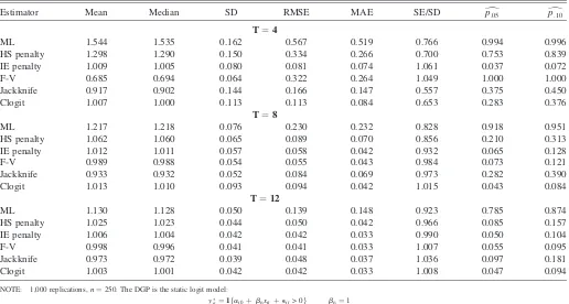
Table 1 displays estimates of the index coefficientb for a static logit model. In addition to ML and penalized likelihood using the HS and IE penalties, we consider the analytic bias correction for binary choice models proposed in Ferna´ndez-Val (2005), the panel jackknife of Hahn and Newey (2004), and the conditional logit estimator of Anderson (1970). We consider panels of lengthT¼4, 8, and 12. Consistent with other studies, ML estimates of the index coefficient b display substantial bias. All of the alternative estimators perform substantially better than ML in estimatingb, in many cases reducing RMSE by over 50% and greatly reducing size distortions in standard hypothesis tests.
For each panel length we consider, the IE penalty and the conditional logit, the latter of which is pffiffiffin-consistent with T
fixed, perform similarly and are superior to the other estimators with the exception of Ferna´ndez-Val (2005) (referred to F-V later and in the tables) withTof 8 or 12 in terms of bias, RMSE, and median absolute error (MAE). The HS penalty also offers a substantial improvement over ML in estimating b, reducing bias by about 50% in theT ¼4 case and 70% in the longer panels. In theT¼4 case, the HS penalty performs similarly in bias and RMSE terms to F-V. While the jackknife performs better than the HS penalty and F-V in the T ¼ 4 case, it is similar to HS and inferior to F-V in the longer panels, and is not
readily generalized to dynamic models. With the exception of the jackknife in theT¼4 case, which has substantial bias for estimating marginal effects, E½@Pðy¼1Þ=@x, all six estima-tors produce very similar estimates of average marginal effects, so we omit these results for brevity.
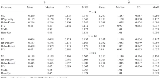
Table 2 displays results for the dynamic logit. We consider estimates ofr, the coefficient on the lagged dependent variable,
yit1, andb, the coefficient on an observed covariate xit. We
report only the HS penalty here as, to our knowledge, the differential equations defining the IE penalty are not soluble in closed form for the dynamic logit. For comparison, we report the bias-corrected estimator proposed in Hahn and Kuersteiner (2004) as well as the bias-corrected estimator for the dynamic logit proposed by Ferna´ndez-Val (2005), and the modified maximum likelihood (MML) estimator in Carro (2006), which is based on a correction of the scores. Because the simulation design is identical, the results for the F-V and MML estimators are taken directly from tables in the respective articles. We also give results for the fixed-T consistent estimator proposed by Honore´ and Kyriazidou (2000b) as reported in Carro (2006). Results for the Hahn-Kuersteiner estimator are based on our own computations and are identical up to Monte Carlo error to results reported in Hahn and Kuersteiner (2004).
For the dynamic logit, we again find that each of the alter-native estimators perform better than the MLE, particularly in estimates ofr where bias is very pronounced. F-V and MML perform comparably to Honore´ and Kyriazidou (2000b). Note that both of these estimators take advantage of the structure of the likelihood in panel discrete choice models in obtaining the
Table 1. Monte Carlo results forb;b static logit
Estimator Mean Median SD RMSE MAE SE/SD dp:05 dp:10
T¼4
ML 1.544 1.535 0.162 0.567 0.519 0.766 0.994 0.996
HS penalty 1.298 1.290 0.150 0.334 0.266 0.700 0.753 0.839
IE penalty 1.009 1.005 0.080 0.081 0.074 1.061 0.037 0.072
F-V 0.685 0.694 0.064 0.322 0.264 1.049 1.000 1.000
Jackknife 0.917 0.902 0.144 0.166 0.147 0.557 0.375 0.450
Clogit 1.007 1.000 0.113 0.113 0.084 0.653 0.283 0.376
T¼8
ML 1.217 1.218 0.076 0.230 0.232 0.828 0.918 0.951
HS penalty 1.062 1.060 0.065 0.089 0.070 0.856 0.210 0.313
IE penalty 1.012 1.011 0.057 0.058 0.042 0.932 0.065 0.128
F-V 0.989 0.988 0.054 0.055 0.043 0.984 0.073 0.121
Jackknife 0.933 0.932 0.052 0.084 0.069 0.973 0.282 0.390
Clogit 1.013 1.010 0.093 0.094 0.042 1.015 0.043 0.084
T¼12
ML 1.130 1.128 0.050 0.139 0.148 0.923 0.785 0.874
HS penalty 1.025 1.023 0.044 0.050 0.042 0.966 0.085 0.157
IE penalty 1.006 1.004 0.042 0.042 0.033 0.990 0.050 0.104
F-V 0.998 0.996 0.041 0.041 0.033 1.007 0.055 0.095
Jackknife 0.973 0.972 0.039 0.048 0.037 1.036 0.097 0.181
Clogit 1.003 1.001 0.042 0.042 0.033 1.008 0.047 0.094
NOTE: 1,000 replications,n¼250. The DGP is the static logit model:
y
it¼1fai0þb0xitþeit> 0g b0¼1
xit;N ð0;p
2
3Þ ai0¼14
P3
t¼0xit eit;Lð0;p
2
3Þ
ML denotes maximum likelihood, HS and IE the penalized ML estimates, using the penalty function (10) and the solution to (8)–(9), respectively. F-V is the bias correction for binary choice models proposed in Ferna´ndez-Val (2005), while CLogit is the conditional logit estimator. RMSE and MAE are the root mean squared error and median absolute deviation from the true values. SE/SD andpb#denotes the average asymptotic standard error divided by SD and empirical rejection frequencies, respectively.
bias-reduction. In this sense, the Hahn-Kuersteiner correction is most comparable to the HS penalty as neither exploits the likelihood nature of the problem or the specific structure of the likelihood. Although the Hahn-Kuersteiner correction outper-forms the HS penalty, the difference in MAE declines quickly as Tincreases and is small relative to the difference between either estimator and the MLE.
The superior performance of F-V and MML relative to the HS penalty and Hahn-Kuersteiner correction suggests that taking advantage of the particular structure of the problem can result in a bias-corrected estimator with better finite sample properties, which has been observed previously in the liter-ature. The IE penalty is another example of this. When it is available, e.g., in the static logit above and the dynamic linear model as considered in Bester and Hansen (2006), it produces an estimator with excellent finite sample properties. However, as implemented here, the IE penalty requires that the expec-tations in (8) and (9) be computed in closed form and the resulting differential equations be soluble analytically, which only occurs in very special cases.
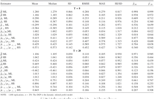
Results for the dynamic ordered probit model are reported in Table 3 for panels of lengthT¼8 and 20. We consider only the HS penalty, as again the IE penalty is not available in closed form. To our knowledge, no explicit analytic bias correction has been proposed in the literature for this model, although some of the other approaches to bias correction mentioned previously could be modified and applied here. However, because the HS penalty depends only on the sample scores and
hessian, it remains easily computed and requires no mod-ification even in a dynamic model with multiple individual specific parameters. For both values ofT, the bias in the ML estimator of b is similar in magnitude to the logit example. Estimates of the coefficients on the lagged outcome,r1 and r1, are severely biased toward zero. In all cases, the HS
penalty provides coefficient estimates that have smaller bias and RMSE than the ML estimates.
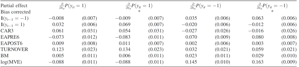
We also consider ML and bias corrected estimates of three marginal effects:
mx¼E @
@xitPðyit¼ 1Þ
m1;1¼E½Pðyit¼1jyit1¼1;Þ Pðyit¼1jyit1¼0;Þ
m1;1¼E½Pðyit¼ 1jyit1¼ 1;Þ Pðyit¼ 1jyit1¼0;Þ:
Bias corrected estimates of these effects are obtained using the approach in Section 2.4. Although both estimates of mx are approximately unbiased, the ML estimates ofm1,1andm1,1
display bias toward zero that, relative to population values, is similar in magnitude to the estimates of the coefficientsr1and r1. We make two observations regarding theT ¼20 panel,
which is the panel length we consider in the empirical appli-cation below. First, our bias correction removes roughly 50% of the bias in the estimates of lagged outcome effects relative to ML. More importantly, size distortions are modest when con-sidering bias corrected marginal effects, which is one of several reasons why we focus on marginal effects when interpreting the results of our empirical application.
Table 2. Monte Carlo results forbrandb;b dynamic logit
b
r bb
Estimator Mean Median SD MAE Mean Median SD MAE
T¼8
ML 0.240 0.240 0.175 0.740 1.260 1.257 0.087 0.260
HS penalty 0.159 0.158 0.155 0.343 1.130 1.130 0.078 0.132
Hahn-Kuerst 0.266 0.266 0.150 0.242 1.081 1.078 0.074 0.090
F-V 0.44 0.43 0.148 0.112 0.99 0.99 0.053 0.037
MML 0.39 0.127 1.01 0.039
Hon-Kyr 0.45 0.131 1.01 0.050
T¼12
ML 0.066 0.068 0.125 0.435 1.147 1.149 0.054 0.147
HS Penalty 0.347 0.348 0.114 0.164 1.052 1.053 0.049 0.059
Hahn-Kuerst 0.400 0.399 0.113 0.125 1.031 1.031 0.047 0.045
F-V 0.47 0.47 0.108 0.073 0.99 0.99 0.053 0.037
T¼16
ML 0.198 0.199 0.104 0.302 1.110 1.110 0.104 0.100
HS Penalty 0.416 0.415 0.098 0.105 1.026 1.026 0.038 0.037
Hahn-Kuerst 0.445 0.445 0.097 0.089 1.014 1.015 0.037 0.032
F-V 0.48 0.47 0.093 0.067 1.00 1.00 0.036 0.024
MML 0.48 0.067 1.01 0.023
Hon-Kyr 0.45 0.074 1.01 0.029
NOTE: 1,000 replications,n¼250. The DGP is the dynamic logit model:
yit¼1fai0þryit1þb0xitþeit> 0g r0¼0:5 b0¼1
xit;N ð0;p
2
3Þ ai0¼14
P3
t¼0xit eit;Lð0;p
2
3Þ
ML denotes maximum likelihood, HS Penalty our penalized ML estimator using the penalty function (10). Hahn-Kuerst is the bias correction proposed in Hahn and Kuersteiner (20,004). F-V is the bias correction for binary choice models proposed in Ferna´ndez-Val (2005), MML is the modified ML estimator proposed in Carro (2006). Hon-Kyr is the fixed-Tconsistent estimator in Honore´ and Kyriazidou (2000b). Results for F-V are taken directly from tables in Ferna´ndez-Val (2005). Results for MML and Hon-Kyr are taken from tables in Carro (2006). Results for Hahn-Kuerst are based on our own computation but appear identical up to Monte Carlo error with those reported in Hahn and Kuersteiner (2004). MAE is the median absolute deviation from the true values.
5. INSIDER TRADING AND EARNINGS ANNOUNCEMENTS
In this section, we apply our penalized likelihood estimator in an empirical study of insider trading activity. We study the extent to which corporate insiders trade on information about how future earnings surprises will affect the firm’s share price, particularly short-term information. Although there is sub-stantial evidence in the literature (e.g., Meulbroek 1992) that insiders trade profitably on nonpublic information before takeovers, empirical evidence on the relationship between insider trading and earnings announcements is mixed, in part due to the difficulties in controlling for the changing regulatory environment and the heterogeneity in incentives faced by insiders at different firms. We attempt to provide some evi-dence on the relationship between insider trading and future returns around earnings announcements dealing with these issues by focusing on a narrow time window with a fairly constant regulatory environment and including firm specific effects to control for differences in incentives across firms. Our analysis complements related work by Roulstone (2006) which makes use of the same data, and we refer the reader there for a more thorough review of the literature on insider trading as well as further details on data sources and variable definitions.
Bias correction is potentially useful in this setting. We will estimate a dynamic nonlinear model with multiple firm specific effects using a panel of firms over a relatively short sample period, and therefore expect that bias will be a large component of estimator risk. In the remainder of this section, we outline the model, provide a brief discussion of the data and variable definitions, and finally present and discuss the results of ML and penalized likelihood estimation.
5.1 Model
The dependent variable is purchases or sales of equity shares by a firm’s corporate insiders (top officers and directors), starting one day after the prior quarter’s earnings announce-ment and ending one day before the current quarter’s announcement. Previous studies in this literature have related the size of insiders’ trades to measures of earnings surprises, which may be problematic for several reasons. First, the data are heavily censored, with 40% of the firm-quarters in our sample having no reported insider activity. Second, the optimal trade size may be a complicated function of insiders’ infor-mation and other factors. For example, a large volume of insider trading may be more likely to attract regulatory atten-tion, particularly when followed by a large unanticipated
Table 3. Monte Carlo results for dynamic ordered probit
Estimator Mean Median SD RMSE MAE SE/SD bp:05 bp:10
T = 8
b
bML 1.280 1.279 0.066 0.288 0.279 0.817 0.998 0.999
b
bHS 1.186 1.185 0.062 0.196 0.185 0.835 0.938 0.972
b
r1ML 0.290 0.289 0.101 0.233 0.211 0.926 0.609 0.712
b
r1HS 0.386 0.387 0.094 0.148 0.116 0.976 0.254 0.360
b
r1ML 0.299 0.298 0.101 0.225 0.202 0.971 0.536 0.659
b
r1HS 0.384 0.385 0.094 0.149 0.115 1.018 0.212 0.312
b
mx=mxML 1.002 1.002 0.053 0.053 0.034 1.517 0.004 0.022
b
mx=mxHS 1.028 1.029 0.055 0.062 0.042 1.329 0.018 0.044
b
m1;1=m1;1ML 0.415 0.411 0.147 0.603 0.589 1.421 0.877 0.946
b
m1;1=m1;1HS 0.624 0.622 0.157 0.407 0.378 1.315 0.428 0.600
b
m1;1=m1;1ML 0.429 0.425 0.145 0.589 0.575 1.727 0.704 0.838
b
m1;1=m1;1HS 0.571 0.573 0.142 0.452 0.427 1.740 0.340 0.542
T = 20
b
bML 1.106 1.105 0.030 0.110 0.105 0.930 0.971 0.985
b
bHS 1.042 1.041 0.028 0.051 0.041 0.962 0.356 0.464
b
r1ML 0.424 0.424 0.054 0.093 0.077 0.952 0.318 0.439
b
r1HS 0.469 0.468 0.052 0.060 0.042 0.985 0.090 0.173
b
r1ML 0.421 0.421 0.056 0.097 0.079 0.957 0.326 0.433
b
r1HS 0.462 0.461 0.054 0.066 0.046 0.991 0.123 0.196
b
mx=mxML 1.013 1.014 0.036 0.038 0.027 1.354 0.009 0.039
b
mx=mxHS 1.012 1.012 0.036 0.038 0.027 1.248 0.024 0.051
b
m1;1=m1;1ML 0.751 0.751 0.099 0.268 0.249 1.052 0.661 0.767
b
m1;1=m1;1HS 0.896 0.897 0.103 0.146 0.108 1.021 0.158 0.253
b
m1;1=m1;1ML 0.744 0.744 0.104 0.276 0.256 1.184 0.548 0.675
b
m1;1=m1;1HS 0.845 0.845 0.103 0.186 0.155 1.198 0.207 0.308
NOTE: 1,000 replications,n¼250. The DGP is the dynamic ordered probit model:
y
it¼ai0þr1;01fyit1¼1gr1;01fyit1¼1gþb0xit þeit yit¼1 y
it> 0
f g 1y
it<ci
f g b0¼1 r1;0¼r1;0¼:5 eit;N ð0;1Þ ai0;N ð1;12Þ
1
6ci0;Betað3;6Þ
The regressorxitfollows a Gaussian AR (1) process withr0¼0.5. Initial conditions arexi0;N ð0;1Þandyi0¼ai0þb0xi0þ N ð0;1Þ. Distributions ofai0andci0were chosen so that
the frequencies ofyitcorrespond approximately with those at the bottom of Table 4. In the table below, ML denotes maximum likelihood, HS the bias corrected estimates using the
penalty function (10). RMSE and MAE are root mean squared error and median absolute deviation of estimates from the true values. SE/SD andpb#denote average asymptotic standard error divided by SD and empirical rejection frequencies, respectively.
earnings surprise. We therefore focus on the sign of net insider activity during a given quarter:yit¼1 denotes net buying by insiders of firmiin quartert,yit¼ 1 denotes net selling, and
yit¼0 denotes no net activity.
We estimate the following ordered probit model:
yit¼ai þ dt þr11fyit1¼1g þ r11fyit1¼ 1g
þbCARit þx9itg þeit
yit¼
1 yit > 0 0 cit<yit #0
1 yit< cit
8 > > < > > :
cit¼ exp ci þdct þr c
11fyit1¼1g þrc11fyit1¼ 1g
þbcCARit þx0itgc; ð15Þ
where CARit, the cumulative abnormal return over the three days1, 0, and 1 relative to the earnings announcement date, is the variable of chief interest;xitis a set of controls discussed below;dtanddtcare period specific effects; andaiandciare time invariant firm specific effects. We note the inclusion of time effects violates the stationarity assumption under which we prove Theorem 1. We drop these effects in one specification later to demonstrate that the results are not sensitive to their inclusion.
The firm specific effects (ai,ci) are present to allow insiders’ decision to trade to depend on unobservable firm-specific factors, including how executive compensation is structured, liquidity, and concerns about legal liability or regulatory attention. The inclusion of multiple effects allows these unobservable factors to affect buying and selling decisions differently. For example, concerns about legal liability may affect selling decisions more than buying decisions, because insider selling ahead of bad news may be more likely to trigger lawsuits against the firm’s management by investors. Similarly, we include two indicators, 1 {yit
1 ¼61} to allow the two
types of insider activity (buying versus selling) to affect the probabilities of insider activity in future quarters in different ways.
In the most general specification we consider, the lower truncation point cit is allowed to depend on the same set of covariates as the linear indexy*, where we note thatcit> 0 is necessary for the model to be sensible. We therefore parame-terize cit as an exponential-linear function of the right side variables. This is done to allow covariates to have asymmetric effects on the probabilities of buying versus selling. For example, ifrc¼bc¼gc¼0, a change in a right side variable that increases the probability of insider buying must also decrease the probability of insider selling. In our empirical analysis later, we find that several of our explanatory variables, includingCAR, enter asymmetrically: Some affect the proba-bility of trading in one direction but not the other, and a few affect the probability of buys and sells in the same direction. Later, we refer to the specification whererc,bc, andgcare free parameters as the asymmetric ordered probit model.
5.2 Data and Variable Definitions
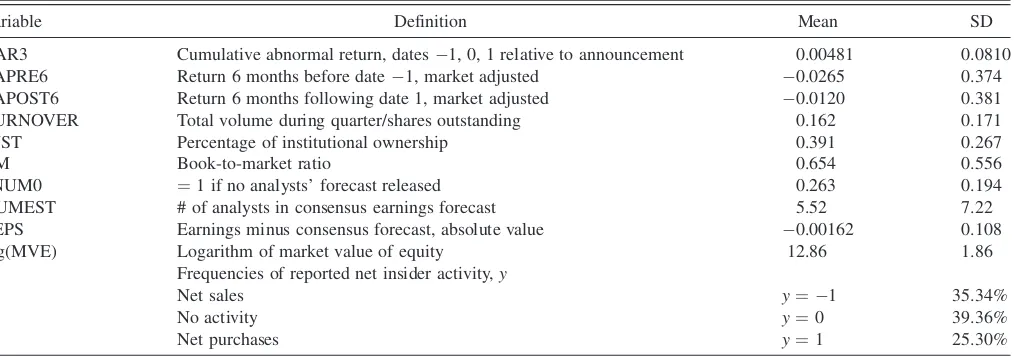
We use a subset of the data considered in Roulstone (2006). The data consist of a quarterly panel of U.S. firms from 1980 to 2002 collected from several sources, including earnings and accounting variables from Compustat; returns, market value, and trading volume from Center for Research in Security Prices (CRSP); and insider purchases and sales from Thompson Financial Insider Trading Data Feed and the National Archives of Insider Trading Summaries. To obtain our subsample, we select firms with one earnings announcement in each quarter from 1996 to 2000. Firms with missing values for any variable are excluded from the sample as are firms with turnover or institutional ownership (both as defined later) greater than 1.5, in part to exclude extreme events such as acquisitions or bankruptcy. We also consider only firms with at least one outcome in each of the three states {1, 0, 1}. The result is a balanced panel with n ¼ 1,213 firms overT ¼20 quarters. Descriptive statistics and a brief summary of variable defi-nitions are provided in Table 4.
Insiders’ decision to trade may be affected by a number of observable factors. As documented by Rozeff and Zaman
Table 4. Descriptive statistics for insider trading data
Variable Definition Mean SD
CAR3 Cumulative abnormal return, dates1, 0, 1 relative to announcement 0.00481 0.0810
EAPRE6 Return 6 months before date1, market adjusted 0.0265 0.374
EAPOST6 Return 6 months following date 1, market adjusted 0.0120 0.381
TURNOVER Total volume during quarter/shares outstanding 0.162 0.171
INST Percentage of institutional ownership 0.391 0.267
BM Book-to-market ratio 0.654 0.556
dNUM0 ¼1 if no analysts’ forecast released 0.263 0.194
NUMEST # of analysts in consensus earnings forecast 5.52 7.22
EEPS Earnings minus consensus forecast, absolute value 0.00162 0.108
log(MVE) Logarithm of market value of equity 12.86 1.86
Frequencies of reported net insider activity,y
Net sales y¼ 1 35.34%
No activity y¼0 39.36%
Net purchases y¼1 25.30%
NOTE: Summary statistics and brief definitions for variables considered in our insider trading application. Our sample consists ofn¼1,213 firms overT¼20 quarters from 1996– 2000. The dependent variable is the sign of net insider activity in the given quarter before the firm’s earnings announcement.
(1998), insider trading activity may depend on past returns and differ across value and growth stocks. Firm size is also potentially important as larger firms are more likely to employ stock-based compensation and the impact of earnings on share price can differ across large and small firms. We therefore include log(MVE), the natural log of the firm’s market value of equity 10 days before the announcement, BM, the book to market ratio, and EAPRE6, the return on the firm’s stock from six months to two days before the announcement minus the market return over the same period, as controls. We include EAPOST6, the excess return on the firm’s stock over the period two days to six months after the announcement, to control for nonearning related future returns. Models of informed trade (e.g., Kyle 1985) predict that insider activity should respond to market volume, prompting us to include TURNOVER, the total trading volume during the quarter divided by shares outstanding.
Finally, the information content of earnings announcements may be influenced by institutional ownership and analyst coverage, prompting us to include INST, EEPS, and NUMEST, respectively, the percentage of institutional ownership, the absolute value of announced earnings per share minus analysts’ consensus forecast, and the number of forecasts in the last I/B/ E/S consensus forecast released before the earnings announcement date. Because a sizable fraction of the firms in our sample have no analyst coverage, we also include a dummy variable dNUM0, which equals one if no consensus forecast was released.
Our analysis complements Roulstone (2006) in several ways. First, to control for changing market conditions and regulatory reform, we focus on a five-year period from 1996 to 2000. This period falls approximately between two important events in insider trading regulation: a 1997 U.S. Supreme Court decision that upheld the SEC’s ability to prosecute trading on the basis of misappropriated nonpublic information, and the release of a detailed set of disclosure regulations by the SEC in late 2000, which were later expanded in the Sarbanes-Oxley
Act of 2002. Roulstone (2006) considers two main specifica-tions, a linear model with firm specific effects and a Tobit model without firm effects and estimates both separately for buys and sells. In this application, the ordered probit specifi-cation allows us to combine information from both types of transactions while accommodating unobserved firm level het-erogeneity in a very flexible way. We also include indicators for buying and selling in the previous quarter and allow each to have asymmetric effects on the probability of insider activity in the current period. Despite the shorter sample period and dif-ferent model specification, our results are qualitatively very similar and the unanticipated earnings announcement return,
CAR, remains statistically significant both before and after bias correction.
5.3 Results and Discussion
We present estimation results for several versions of the ordered probit model (15) using the data discussed previously. We estimate all models considered by ML. For models with individual specific effects, we also present penalized likelihood estimates using the penalty function given in Equation (10), which are free fromOð1=TÞbias, as discussed in Section 2.
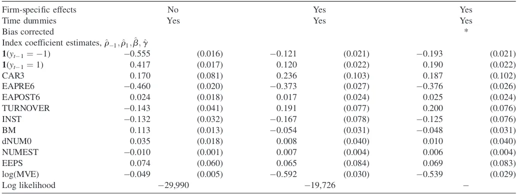
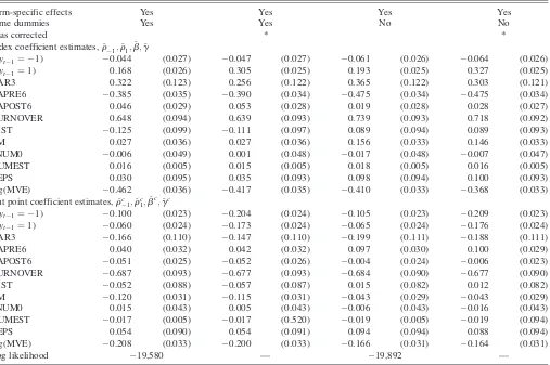
We first consider a standard ordered probit model, as given in (15) with the additional restrictionsrc¼bc¼gc¼0. The left and center columns of Table 5 present ML estimates and standard errors for this model, respectively, without and with firm specific fixed effects. Bias corrected estimates for the model with fixed effects are presented in the right columns of the table. These estimates highlight two important features of our data and estimation procedure. First, unobserved firm-level heterogeneity plays a prominent role. Controlling for firm specific heterogeneity has a large impact on the coefficients on the lagged outcomes,1{yit
1¼1} and1{yit1¼ 1}. Book to
market and analyst coverage are no longer statistically sig-nificant after fixed effects are added. Also, for the fixed effects specification, our bias correction has a substantial impact on
Table 5. Ordered probit estimates for insider trading data
Firm-specific effects No Yes Yes
Time dummies Yes Yes Yes
Bias corrected *
Index coefficient estimates,r^1;^r1;b;^ g^
1(y
t1¼ 1) 0.555 (0.016) 0.121 (0.021) 0.193 (0.021)
1(yt1¼1) 0.417 (0.017) 0.120 (0.022) 0.190 (0.022)
CAR3 0.170 (0.081) 0.236 (0.103) 0.187 (0.102)
EAPRE6 0.460 (0.020) 0.373 (0.027) 0.376 (0.026)
EAPOST6 0.024 (0.018) 0.017 (0.024) 0.025 (0.024)
TURNOVER 0.143 (0.041) 0.191 (0.077) 0.200 (0.076)
INST 0.132 (0.032) 0.167 (0.078) 0.125 (0.076)
BM 0.113 (0.013) 0.054 (0.031) 0.048 (0.031)
dNUM0 0.035 (0.018) 0.008 (0.040) 0.010 (0.040)
NUMEST 0.010 (0.001) 0.007 (0.004) 0.006 (0.004)
EEPS 0.074 (0.060) 0.065 (0.084) 0.069 (0.083)
log(MVE) 0.049 (0.005) 0.592 (0.030) 0.539 (0.029)
Log likelihood 29,990 19,726
NOTE: Ordered probit parameter estimates for our insider trading application. The model is as in Equation (15) with the restrictionsrc
1¼rc1¼bc¼gc¼0 imposed. Standard errors
are shown in parentheses. The left columns show estimates with no firm-specific effects. The center and right columns show estimates with two firm-specific effects before and after bias correction. Variable definitions are given in Table 3.