NOSQL FOR STORAGE AND RETRIEVAL OF LARGE LIDAR DATA COLLECTIONS
J. Boehm, K. Liu
Department of Civil, Environmental & Geomatic Engineering, University College London, Gower Street, London, WC1E 6BT UK – [email protected]
Commission III, WG III/5
KEY WORDS: LiDAR, point cloud, database, spatial query, NoSQL, cloud storage
ABSTRACT:
Developments in LiDAR technology over the past decades have made LiDAR to become a mature and widely accepted source of geospatial information. This in turn has led to an enormous growth in data volume. The central idea for a file-centric storage of LiDAR point clouds is the observation that large collections of LiDAR data are typically delivered as large collections of files, rather than single files of terabyte size. This split of the dataset, commonly referred to as tiling, was usually done to accommodate a specific processing pipeline. It makes therefore sense to preserve this split. A document oriented NoSQL database can easily emulate this data partitioning, by representing each tile (file) in a separate document. The document stores the metadata of the tile. The actual files are stored in a distributed file system emulated by the NoSQL database. We demonstrate the use of MongoDB a highly scalable document oriented NoSQL database for storing large LiDAR files. MongoDB like any NoSQL database allows for queries on the attributes of the document. As a specialty MongoDB also allows spatial queries. Hence we can perform spatial queries on the bounding boxes of the LiDAR tiles. Inserting and retrieving files on a cloud-based database is compared to native file system and cloud storage transfer speed.
1. INTRODUCTION
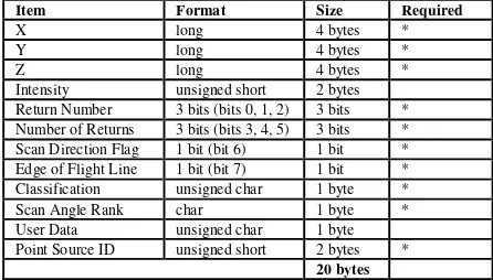
Current workflows for LiDAR point cloud processing often involve classic desktop software packages or command line interface executables. Many of these programs read one or multiple files, perform some degree of processing and write one or multiple files. Examples of free or open source software collections for LiDAR processing are LASTools (Isenburg and Schewchuck, 2007) and some tools from GDAL (“GDAL - Geospatial Data Abstraction Library,” 2014) and the future PDAL (“PDAL - Point Data Abstraction Library,” 2014). Files have proven to be a very reliable and consistent form to store and exchange LiDAR data. In particular the ASPRS LAS format (“LAS Specification Version 1.3,” 2009) has evolved into an industry standard which is supported by every relevant tool. For more complex geometric sensor configurations the ASTM E57 (Huber, 2011) seems to be the emerging standard. For both formats open source, royalty free libraries are available for reading and writing. There are now also emerging file standards for full-waveform data. File formats sometimes also incorporate compression, which very efficiently reduces overall data size. Examples for this are LASZip (Isenburg, 2013) and the newly launched ESRI Optimized LAS (“Esri Introduces Optimized LAS,” 2014). Table 1 shows the compact representation of a single point in the LAS file format (Point Type 0). Millions of these 20 byte records are stored in a single file. It is possible to represent the coordinates with a 4 byte integer, because the header of the file stores an offset and a scale factor, which are unique for the whole file. In combination this allows a LAS file to represent global coordinates in a projected system.
This established tool chain and exchange mechanism constitutes a significant investment both from the data vendors and from a data consumer side. Particularly where file formats are made open they provide long-term security of investment and provide maximum interoperability. It could therefore be highly attractive to secure this investment and continue to make best use of it.
However, it is obvious that the file-centric organization of data is problematic for very large collections of LiDAR data as it lacks scalability.
2. LIDAR POINT CLOUDS AS BIG DATA
Developments in LiDAR technology over the past decades have made LiDAR to become a mature and widely accepted source of geospatial information. This in turn has led to an enormous growth in data volume. For airborne LiDAR a typical product today which can be bought form a data vendor is a 25 points per square meter point cloud stored in a LAS file. This clearly exceeds by an order of magnitude a 1 meter DEM raster file, which was a GIS standard product not so long ago. Not only did the point count per square meter increase but the extent in the collection of data has significantly increased as well.
As an example we can use the official Dutch height network (abbreviated AHN), which has recently been made publicly available (“AHN - website,” 2014). The Netherlands extend across approximately 40,000 square kilometres (including water surfaces). At 25 points per square meter or 25,000,000 points per
Item Format Size Required
X long 4 bytes *
Y long 4 bytes *
Z long 4 bytes *
Intensity unsigned short 2 bytes Return Number 3 bits (bits 0, 1, 2) 3 bits * Number of Returns 3 bits (bits 3, 4, 5) 3 bits * Scan Direction Flag 1 bit (bit 6) 1 bit * Edge of Flight Line 1 bit (bit 7) 1 bit * Classification unsigned char 1 byte * Scan Angle Rank char 1 byte * User Data unsigned char 1 byte Point Source ID unsigned short 2 bytes *
20 bytes
Table 1: Compact representation of a single point in the LAS file format.
square kilometre a full coverage could theoretically result in ∙
6∙ ∙ = or one trillion points. At 20 bytes each this
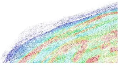
truly constitutes big data. The current AHN2 covers less ground and provides an estimated 400 billion points (Swart, 2010). It delivers more than 1300 tiles of about one square kilometre each of filtered terrain-only points at an average density of 10 points per square meter. The same volume is available for the residual filtered out points (e.g. vegetation and buildings). Together this is over a terabyte of compressed data in more than 2500 files. Figure 1 shows a single tile of that dataset. It is one of the smallest tiles of the dataset. The single tile contains 56,603,846 points and extends from 141408.67 to 145000.00 in Easting and 600000.00 to 601964.94 in Northing. In compressed LAZ format it uses 82 MB disk space and uncompressed it uses 1.05 GB.
In terrestrial mobile scanning acquisition rates have now surpassed airborne acquisition rates and therefore data volumes can become even larger. Organization such as public transport authorities are scanning their tunnel systems in regular intervals for inspection and monitoring purposes. Repetitive acquisitions at centimetre and even millimetre spacing result in large collections which accumulate over the years. In order to detect changes over several epochs data from previous acquisitions needs to be available just as well as the most recent acquisition. These examples clearly demonstrate the tough requirements on data storage, redundancy, scalability and availability for LiDAR storage. Just as clearly traditional file-centric organization of data faces some challenges to meet these requirements. However databases have dealt with these requirements successfully for years.
3. POINT CLOUDS AND DATABASES
The simplest approach to store LiDAR point clouds in a relational database, would be to store every point in a row of a three column table where the columns represent X, Y and Z. Further columns could represent additional attributes (see Table 1). As (Ramsey, 2013) has mentioned classic relational databases are not cable to store hundreds of billions of rows for performance reasons. However, this would be necessary as follows from the examples above. Classic databases can maybe store millions of rows. There have been nevertheless efforts to approach this. The solution is typically to collect a larger set of points and store them as a single object in a row. The two major examples for this are Oracle Spatial and PostGIS. PostGIS refers to this concept as point cloud patches (PcPatch). The obvious disadvantage is that to access the actual geometry, i.e. the individual points you need to unpack these patches (PC_Explode) and casted to classic GIS points, which is an additional operation. For PostGIS the recommendation is to use patches with a maximum of 600 points, i.e. rather small patches.
Google’s Bigtable (Chang et al., 2008) finally promised to break the storage boundaries of traditional databases. According to the authors Bigtable was designed as a distributed database system to hold “petabytes of data across thousands of commodity servers”. The number of rows in a database is virtually unlimited. A Bigtable inspired open source distributed database system HBase was used as a storage backend for Megatree (“Megatree - ROS Wiki,” 2008). Megatree is an octree like spatial data structure to hold billions of points. It is now maintained by hiDOF (“hiDOF,” 2014).
Document oriented NoSQL (Not only SQL) databases depart from the idea of storing data in tables. A significant portion of NoSQL databases (mongodb, couchbase, clusterpoint …) are indeed document oriented (Jing Han et al., 2011). If one was to draw a comparison to relational databases documents were the equivalent to rows in a table. A collection of documents then makes up the table. The decisive difference is that the documents in a collection need not follow the same schema. They can contain different attributes while the database is still able to query across all documents in a collection. These NoSQL databases are highly scalable and are one of the most significant tools for Big Data problems. We introduce a possible solution for LiDAR storage using NoSQL that follows a file-centric approach in the following section. We had first suggested the use of document oriented NoSQL for LiDAR storage in (Boehm, 2014). (Wang and Hu, 2014) have proposed a similar approach focusing on concurrency.
4. NOSQL DATABASE FOR FILE-CENTRIC STORAGE
The central idea for a file-centric storage of LiDAR point clouds is the observation that large collections of LiDAR data are typically delivered as large collections of files, rather than single files of terabyte size. This split of the dataset, commonly referred to as tiling, was usually done to accommodate a specific processing pipeline. It makes therefore sense to preserve this split.
A document oriented NoSQL database can easily emulate this data partitioning, by representing each tile (file) in a separate document. The document stores the metadata of the tile. Different file formats could be accommodated by different attributes in the document, as NoSQL does not enforce a strict schemata. The actual files cannot efficiently be stored inside a document as they are too large. A different mechanism is needed.
We choose to use MongoDB a highly scalable document oriented NoSQL database. MongoDB offers GridFS which emulates a distributed file system. This brings the possibility to store large LiDAR files over several servers and thus ensures scalability. GridFS is a database convention to enable file storage. A file is split up into smaller chunks which are stored in separate documents linked via a common id. An index keeps track of the chunks and stores the associated file attributes. The idea to store large geospatial collections in a distributed file system is not dissimilar to Spatial Hadoop which uses HDFS for this purpose (Eldawy and Mokbel, 2013). Figure 2 gives an overview of the proposed architecture of the database. Figure 3 details the attributes that are stored in a document. Note that this is not meant to be a fixed schema, it is rather a minimal set of information which can be easily extended.
Figure 1: Visualization of a single point cloud tile stored in a LAS file. The colours indicate height.
Figure 2: Overview of the three collections that make up the database for big LiDAR data
{
type: <file type, e.g. LAS>,
version: <version of file format>,
id: <project id>,
date: <acquisition date>,
loc: <location for spatial index>,
filename: <original file name>,
gridfs_id: <pointer to gridfs file>
}
Figure 3: Attributes of a document stored in the collection representing the metadata of a tile.
5. IMPLEMENTATION DETAILS
We start from the data provided by the LAS files. The information in their headers provides the crucial metadata for later queries. We use liblas (Butler et al., 2010) and its python bindings to parse the files. While we show all code excerpts in python for brevity there is nothing language specific in the data organization. The following python code excerpt shows an example of metadata that can be extracted. In this example we use the file’s signature, the version of LAS, the project ID and the date to describe the file’s content. We also extract the minimum and maximum of coordinate values to later construct the bounding box.
# open LAS/LAZ file
file_name = 'g01cz1.laz'
f = file.File(file_name, mode='r')
header = f.header
# read meta data from header
s = header.file_signature
v = header.version
i = header.project_id
d = header.date
min = header.min
max = header.max
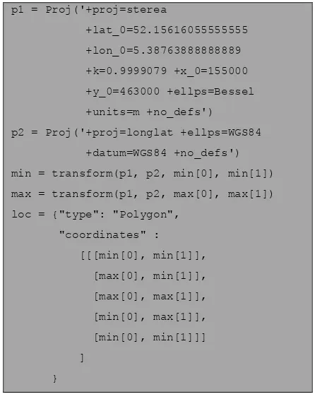
Many of the NoSQL databases target web and mobile development. Hence their geospatial indices are often restricted to GPS coordinates, which are most commonly represented in WGS84. LiDAR data on the other hand is usually locally projected. Therefore any coordinates extracted from a LiDAR
file need to me transformed to the correct coordinate system supported by the database. This is a very common operation in GIS. We use the PROJ library for this purpose. Again we provide some sample code which shows the transformation from the original coordinate systems (Amersfoort / RD New to WGS84 in this case). As you can see we only transform the bounding box of the data. The actual LiDAR data remains untouched.
p1 = Proj('+proj=sterea
+lat_0=52.15616055555555
+lon_0=5.38763888888889
+k=0.9999079 +x_0=155000
+y_0=463000 +ellps=Bessel
+units=m +no_defs')
p2 = Proj('+proj=longlat +ellps=WGS84
+datum=WGS84 +no_defs')
min = transform(p1, p2, min[0], min[1])
max = transform(p1, p2, max[0], max[1])
loc = {"type": "Polygon",
"coordinates" :
[[[min[0], min[1]],
[max[0], min[1]],
[max[0], max[1]],
[min[0], max[1]],
[min[0], min[1]]]
]
}
For all of the above the actual data content of the LiDAR file never gets analysed. This is important to avoid unnecessary overhead. The file gets stored in full and unaltered into the database. As mentioned above MongoDB provides a distributed file system for this called GridFS. We show in following code how the compressed LAS file gets stored into the database. We store a pointer to the file (a file ID) to connect it to the metadata in the next step.
We have now all the information in place to generate a document which combines the meta data of the LiDAR file, the geometric key and a pointer to the actual data content in the database (see Figure 3). This NoSQL document represents one tile of the collection of LiDAR data. The document is represented as a BSON object. This representation is very similar to the well-known JSON representation, but optimized for storage. The actual creation of the document and its storage are very simple. The next code sample shows all that is required.
Database
collections
big_lidar
tile metadata
fs.files
file attributes
fs.chunks
file chunks
# open mongodb big_lidar database
client = MongoClient()
db = client.test_database
big_lidar = db.big_lidar
# add file to GridFS
file = open(file_name, 'rb')
gfs = gridfs.GridFS(db)
gf = gfs.put(file, filename = file_name)
file.close()
# add one tile to big_lidar database
tile = {"type": s, "version": v, "id": i,
"date": d, "loc": loc,
"filename": file_name,
"gridfs_id": gf}
big_lidar.insert(tile)
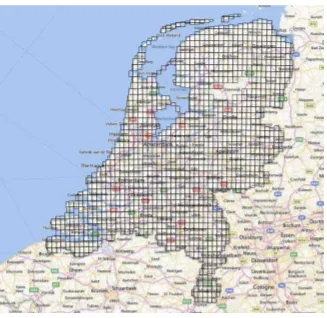
Figure 4 shows a graphical result of the operation. It is the visualization of all stored tiles’ bounding boxes on top of a map using a desktop GIS system (Quantum GIS). Since the bounding boxes are stored as BSON objects, it is straight forward to export them as GeoJSON files.
We show a simple status report and an aggregation on the database in the MongoDB console. This confirms the successful
storage of 1351 tiles and a total of 447728000747 points in the database.
> db.big_lidar.stats()
{
"ns" : "AHN2.big_lidar",
"count" : 1351,
"size" : 670096,
"avgObjSize" : 496,
"storageSize" : 696320, …
}
> db.big_lidar.aggregate( [ { $group : { _id:
null, total: { $sum : "$num_points" } } } ] )
{ "_id" : null, "total" :
NumberLong("447728000747") }
6. SPATIAL QUERY
MongoDB like any NoSQL database allows for queries on the attributes of the document. When an index is created on a certain attribute queries are accelerated. As a specialty MongoDB allows spatial indices and spatial queries. Hence we can perform spatial
Figure 4: Bounding Polygons of the tiles of the AHN2 dataset displayed over a map.
queries on the bounding boxes of the LiDAR tiles. We show a very simple example of an interactive query on the Python console. The query uses a polygon to describe the search area. The database returns the tile metadata including the GridFS index. Using the GridFS index the actual point cloud data can be read from the database. It is simply the LiDAR point cloud file that was previously put into the database. It is important to note that no conversion or alteration of the files was done.
>>> tiles=list(big_lidar.find({ "loc" :
{ "$geoWithin" : { "$geometry" :
{"type": "Polygon", "coordinates" :
[[[5.1, 53.3], [5.5, 53.3],
[5.5, 53.5], [5.1, 53.5],
[5.1, 53.3] ]]}}}
}))
>>> len(tiles)
4
>>> tiles[0]['filename']
u'g01cz1.laz'
>>> gf_id = tiles[0]['gridfs_id']
>>> gf = gfs.get(gf_id)
>>> las_file = open('export_' + file_name,
'wb')
>>> las_file.write(gf.read())
>>> las_file.close()
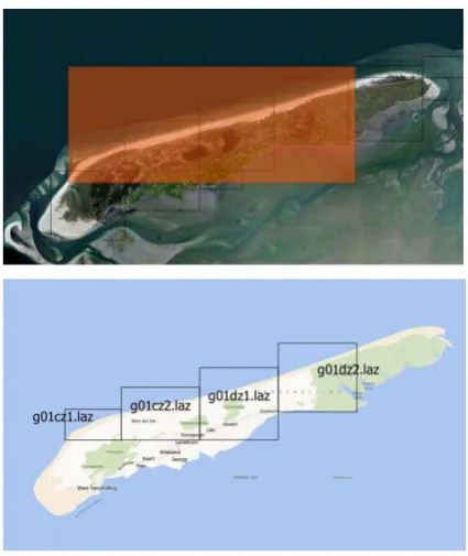
In Figure 5 we give the visualization representation of the query operation. Four tiles were retrieved by the spatial query. In the example we attach the filename as attributes and plot the bounding boxes over a base map using the filenames as labels. The leftmost tile corresponds to the point cloud visualized in Figure 1.
7. TIMING EXPERIMENTS
As we move file-centric storage from the operating systems’ file systems to a database, the performance of the transfer operation with respect to the time they need to complete is of interest. We have therefore performed some timing experiments for simple storage and retrieval of a single tile of about 40 MB. The experiments were performed on an Amazon EC2, a well-known high-performance computing environment (Akioka and Muraoka, 2010). We used an EC2 small instance in all experiments. We separated local transfer from remote transfer. Local Transfer is in-between the operating systems’ file system and the database on the same machine. Remote transfer occurs between the EC2 instance and a machine outside the amazon cluster connected via the internet. To better assess the measured times we give comparisons to alternative transfer methods. We compare local transfer to the timing measured for direct file system transfer (file-copy). Remote transfer is compared to transfer with Dropbox, a leading personal cloud storage service (Drago et al., 2012).
Figure 6 shows the results of local transfer. We can see that there is some overhead compared to file system copy. This is particularly the case for storing files (put), less so for retrieving
them (get). Figure 7 shows the timings for remote transfer. The database performs at least on par with a common cloud storage system. This obviously depends on the internet connection. All experiments were performed on the same computers at nearly the same time.
Figure 6: Transfer times for local transfer.
Figure 7: Transfer times for remote transfer.
0.036
1.515 0.268
0.000 0.500 1.000 1.500 2.000 OS file copy
GridFS - put GridFS - get
Local Transfer (~40MB Tile) in sec.
95.8 116.1 6.2
13.1
0.0 50.0 100.0 150.0
GridFS - upload Dropbox - upload GridFS -download Dropbox - download
Remote Transfer (~40MB Tile) in sec.
Figure 5: Example result of a spatial query visualized using QGIS. In the top image the red box represents the search polygon. The bottom image shows the tiles that are completely within the search polygon. The MongoDB spatial query delivered four tiles on the coast of the Netherlands.
8. CONCLUSIONS
We have presented a file-centric storage and retrieval system for large collections of LiDAR point cloud tiles based on scalable NoSQL technology. The system is capable of storing large collections of point clouds. Using a document-based NoSQL database allows retaining a file-centric workflow, which makes many existing tools accessible. The suggested system supports spatial queries on the tile geometry. Inserting and retrieving files locally has some overhead when compared to file system operation. Remote transfer is at par with popular cloud storage. Building the system on MongoDB, a proven NoSQL database, brings in a range of advantageous features such as
Scalability Replication High Availability Auto-Sharding
MongoDB supports Map-Reduce internally for database queries. However it is also known to work with external Map-Reduce frameworks such as Hadoop. A special adapter to access MongoDB from Hadoop is provided. This offers very interesting future opportunities to combine Map-Reduce based processing with NoSQL spatial queries.
9. ACKNOWLEDGEMENTS
We would like to acknowledge that this work is in part supported by an Amazon AWS in Education Research Grant award. Also part of this work is supported by EU grant FP7-ICT-2011-318787 (IQmulus).
REFERENCES
AHN - website [WWW Document], 2014. URL http://-www.ahn.nl/index.html (accessed 5.19.14).
Akioka, S., Muraoka, Y., 2010. HPC Benchmarks on Amazon EC2. IEEE, pp. 1029–1034. doi:10.1109/WAINA.2010.166 Boehm, J., 2014. File-centric organization of large LiDAR Point Clouds in a Big Data context.
Butler, H., Loskot, M., Vachon, P., Vales, M., Warmerdam, F., 2010. libLAS: ASPRS LAS LiDAR Data Toolkit [WWW Document]. libLAS - LAS 1.0/1.1/1.2 ASPRS LiDAR data translation toolset. URL http://www.liblas.org/
Chang, F., Dean, J., Ghemawat, S., Hsieh, W.C., Wallach, D.A., Burrows, M., Chandra, T., Fikes, A., Gruber, R.E., 2008. Bigtable: A distributed storage system for structured data. ACM Transactions on Computer Systems (TOCS) 26, 4.
Drago, I., Mellia, M., M. Munafo, M., Sperotto, A., Sadre, R., Pras, A., 2012. Inside dropbox: understanding personal cloud storage services. ACM Press, p. 481. doi:10.1145/2398776.-2398827
Eldawy, A., Mokbel, M.F., 2013. A demonstration of SpatialHadoop: an efficient mapreduce framework for spatial data. Proceedings of the VLDB Endowment 6, 1230–1233. Esri Introduces Optimized LAS [WWW Document], 2014. URL http://blogs.esri.com/esri/arcgis/2014/01/10/esri-introduces-optimized-las/ (accessed 5.19.14).
GDAL - Geospatial Data Abstraction Library [WWW Document], 2014. URL http://www.gdal.org/ (accessed 9.4.14). hiDOF [WWW Document], 2014. URL http://hidof.com/ Huber, D., 2011. The ASTM E57 file format for 3D imaging data exchange, in: IS&T/SPIE Electronic Imaging. International Society for Optics and Photonics, p. 78640A–78640A.
Isenburg, M., 2013. LASzip: lossless compression of LiDAR data. Photogrammetric Engineering and Remote Sensing 79, 209–217.
Isenburg, M., Schewchuck, J., 2007. LAStools: converting, viewing, and compressing LIDAR data in LAS format. avaliable at: http://www. cs. unc. edu/ isenburg/lastools.
Jing Han, Haihong E, Guan Le, Jian Du, 2011. Survey on NoSQL database. IEEE, pp. 363–366. doi:10.1109/ICPCA.2011.-6106531
LAS Specification Version 1.3, 2009.
Megatree - ROS Wiki [WWW Document], 2008. URL http://-wiki.ros.org/megatree
PDAL - Point Data Abstraction Library [WWW Document], 2014. URL http://www.pdal.io/ (accessed 9.4.14).
Ramsey, P., 2013. LIDAR In PostgreSQL With Pointcloud. Swart, L.T., 2010. How the Up-to-date Height Model of the Netherlands (AHN) became a massive point data cloud. NCG KNAW 17.
Wang, W., Hu, Q., 2014. The Method of Cloudizing Storing Unstructured LiDAR Point Cloud Data by MongoDB, in: Geoinformatics (GeoInformatics), 2014 22nd International Conference on, Kaohsiung, Taiwan, China. pp. 1–5. doi:10.1109/GEOINFORMATICS.2014.6950820