FAST SEMANTIC SEGMENTATION OF 3D POINT CLOUDS WITH STRONGLY
VARYING DENSITY
Timo Hackel, Jan D. Wegner, Konrad Schindler
Photogrammetry and Remote Sensing, ETH Z¨urich – [email protected]
Commission III, WG III/2
KEY WORDS:Semantic Classification, Scene Understanding, Point Clouds, LIDAR, Features, Multiscale
ABSTRACT:
We describe an effective and efficient method for point-wise semantic classification of 3D point clouds. The method can handle unstructured and inhomogeneous point clouds such as those derived from static terrestrial LiDAR or photogammetric reconstruction; and it is computationally efficient, making it possible to process point clouds with many millions of points in a matter of minutes. The key issue, both to cope with strong variations in point density and to bring down computation time, turns out to be careful handling of neighborhood relations. By choosing appropriate definitions of a point’s (multi-scale) neighborhood, we obtain a feature set that is both expressive and fast to compute. We evaluate our classification method both on benchmark data from a mobile mapping platform and on a variety of large, terrestrial laser scans with greatly varying point density. The proposed feature set outperforms the state of the art with respect to per-point classification accuracy, while at the same time being much faster to compute.
1. INTRODUCTION
Dense 3D acquisition technologies like laser scanning and auto-mated photogrammetric reconstruction have reached a high level of maturity, and routinely deliver point clouds with many mil-lions of points. Due to their lack of structure, raw point clouds are of limited use for downstream applications beyond visual-ization and simple distance measurements, therefore much effort has gone into developing automated approaches for point cloud interpretation. The two main tasks are on the one hand to derive semantic information about the scanned objects, and on the other hand to convert point clouds into higher-level, CAD-like geomet-ric representations. Both tasks have turned out to be surprisingly difficult to automate.
In this work we are concerned with the first problem. Much like in semantic image segmentation (a.k.a. pixel labelling), we at-tempt to attach a semantic label to every single 3D point. Point-wise labels areper sealso not a final result. But like several other authors, e.g. (Golovinskiy et al., 2009, Lafarge and Mallet, 2012), we argue that it makes sense to extract that information at an early stage, in order to support later processing steps. In particular, se-mantic labels (respectively, soft class probabilities) allow one to utilize class-specific a-priori models for subsequent tasks such as surface fitting, object extraction, etc.
Early work on semantic segmentation of airborne LiDAR data aimed to classify buildings, trees and the ground surface, and sometimes also to reconstruct the buildings. In many cases the point cloud is first converted to a heightfield, so that standard image processing methods can be applied, e.g. (Hug and Wehr, 1997, Haala et al., 1998). More recent work in aerial imaging has followed the more general approach to directly label 3D points, using geometric information derived from a set of neighbors in the point cloud, e.g. (Chehata et al., 2009, Yao et al., 2011). 3D point labelling is also the standard method for terrestrial mo-bile mapping data, for which it is not obvious how to generate a consistent 2.5-dimensional height (respectively, range) map, e.g. (Golovinskiy et al., 2009, Weinmann et al., 2013). Like many other recent works we follow the standard pipeline of discrimina-tive classification: First, extract a rich, expressive set of features
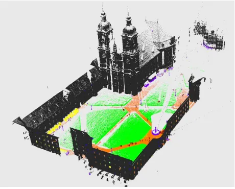
Figure 1. The task: given an unstructured, inhomogeneous point cloud, assign point-wise semantic labels.
that capture the geometric properties of a point’s neighborhood. Then, train an off-the-shelf classifier to predict class-conditional probabilities from those features.
Compared to existing work, we aim to handle all kinds of scan data, including point clouds from static terrestrial laser scanning (TLS) or close-range photogrammetry. Due to the measurement principle (polar recording from a limited number of instrument locations), this type of data exhibits huge variations in point den-sity. First of all, point density naturally decreases quadratically with distance. Second, the laser intensity (respectively, for image-based reconstruction the amount of accurately localisable surface detail) also decreases with distance, so that more points do not generate a return at all. Third, the setup with few viewpoints from close range makes it all but impossible to avoid large occlusions.
not involve expensive computations: if one uses 1 millisecond per point, it already takes approximately 3 hours to classify 10 million points. The contribution of the present paper is a feature set that addresses both variations in point density and computa-tional efficiency. We propose variants and approximations of a number of existing features to capture the geometry in a point’s local neighborhood. Central to the improved feature definitions is the concept ofneighborhood. By appropriately chosing which nearby points form the basis for computing features at different scales, the proposed method(i)is robust against strong variations of the local point density, respectively point-to-point distance; and (ii)greatly speeds up the pointwise feature extraction that constitutes the computational bottleneck.
We present experimental evaluations on several different datasets from both mobile mapping and static terrestrial LiDAR, see Fig-ure 1. ForParis-Rue-Cassetteand Paris-Rue-Madamethe pro-posed method reaches overall classification accuracies of 95-98% at a mean class recall 93-99%, to our knowledge the best results reported to date. The end-to-end computation time of our system on these datasets is<4minutes per 10 million points, compared to several hours reported in previous work.
2. RELATED WORK
Semantic segmentation of point clouds has mostly been inves-tigated for laser scanner data captured from airplanes, mobile mapping systems, and autonomous robots. Some of the earli-est work on point cloud classification dealt with airborne LiDAR data, with a focus on separating buildings and trees from the ground surface, and on reconstructing the buildings. Often the point cloud is converted to a regular raster heightfield, in order to apply well-known image processing algorithms like edge and texture filters for semantic segmentation (Hug and Wehr, 1997), usually in combination with maximum likelihood classification (Maas, 1999) or iterative bottom-up classification rules (Haala et al., 1998, Rottensteiner and Briese, 2002). Given the focus on buildings, another natural strategy is to model them with a lim-ited number of geometric 2D (Schnabel et al., 2007, Pu and Vos-selman, 2009) or 3D (Li et al., 2011, Xiao and Furukawa, 2014) primitives, which are fitted to the points – see also (Vosselman et al., 2004) for an overview of early work. A limitation of such methods is that for most realistic scenes a fixed shape library is insufficient. It has thus been proposed to fill the remaining gaps with unstructured triangle meshes, generated by triangulat-ing the raw points (Lafarge and Mallet, 2012). Recent work in aerial imaging has followed the more general strategy also used in this paper, namely to first attach semantic meaning to individ-ual points through supervised classification, and then continue high-level modelling from there (Charaniya et al., 2004, Chehata et al., 2009, Niemeyer et al., 2011, Yao et al., 2011). Also re-lated to that strategy are methods for classifying tree species in forestry, e.g. (Orka et al., 2012, Dalponte et al., 2012).
A second main application area is the semantic classification of point clouds acquired with mobile mapping systems, sometimes in combination with airborne LiDAR (Kim and Medioni, 2011); to extract for example roads (Boyko and Funkhouser, 2011), build-ings (Pu et al., 2011), street furniture (Golovinskiy et al., 2009) or trees (Monnier et al., 2012). Several authors solve for all relevant object classes at once, like we do here, by attaching a label to ev-ery single 3D point (Weinmann et al., 2013, Dohan et al., 2015). Related work in robotics uses point classification to separate the ground from trees and other obstacles (Lalonde et al., 2006).
At the heart of point-wise semantic labelling is the task of de-signing appropriate features (descriptors), which capture the ge-ometric properties of a point’s neighborhood such as roughness,
surface orientation, height over ground, etc. A large variety of geometric 3D point descriptors exist. Among the most popu-lar ones are spin images (Johnson and Hebert, 1999), fast point feature histograms (FPFH) (Rusu et al., 2009) and signatures of histograms (SHOT) (Tombari et al., 2010). These methods were originally developed as descriptors for sparse keypoints, and while they do work well also as dense features for point labelling, they tend to be expensive to compute and thus do not scale well to large point clouds. Features designed for dense point cloud de-scription are often based on the structure tensor of a point’s neigh-borhood (Demantk´e et al., 2011), custom descriptors for vertical cylindrical shapes (Monnier et al., 2012) and the height distri-bution in a vertical column around the point (Weinmann et al., 2013). Some authors have tried to avoid the analysis of the struc-ture tensor to describe shape, e.g. by characterising the shape with a randomised set of histograms (Blomley et al., 2014). In our ex-perience this does not improve the results, but has significantly higher runtime. For speech and image understanding, end-to-end feature learning with convolutional neural networks (CNNs) has in the last few years become a de-facto standard. To our knowl-edge, it has only been used – with some success – for 3D voxel grids (Lai et al., 2014, Wu et al., 2015), but not yet for generic point clouds; Presumably because the convolutional strategy is not efficient in the absence of a regular neighborhood structure.
We found that features derived from the structure tensor and the vertical point distribution work well over a wide range of scales, and are particularly fast when combined with an efficient approxi-mation of a point’s multi-scale neighborhood (Pauly et al., 2003). Our proposed feature extraction can thus be seen as a fast multi-scale extension of (Weinmann et al., 2013). A common strategy to account for correlations between class labels (e.g. smoothness, or frequent neighborhood patterns) is to use the point-wise class probabilities as unary term in some sort of random field model. This has also been tried for point cloud classification. For exam-ple, (Shapovalov et al., 2010) propose a non-associative Markov random field for semantic 3D point cloud labelling, after a pre-segmentation of the point cloud into homogeneous 3D segments. (Najafi et al., 2014) follow the same idea and add higher-order cliques to represent long-range correlations in aerial and mobile mapping scans of cities. (Rusu et al., 2009) use FPFH together with a Conditional random field (CRF) to label small indoor Li-DAR point clouds. (Niemeyer et al., 2011, Schmidt et al., 2014) use a CRF with Random Forest unaries to classify urban objects, respectively land-cover in shallow coastal areas. In the present work we do not model correlations between points explicitly. However, since our method outputs class-conditional probabil-ities for each point, it is straight-forward to combine it with a suitable random field prior. We note, however, that at least local Potts-type interactions would probably have at most a small ef-fect, because smoothness is implicitly accounted for by the high proportion of common neighbors shared between nearby points. On the other hand, inference is expensive even in relatively sim-ple random field models. To remain practical for real point clouds one might have to ressort to local tiling schemes, or approximate inference with fast local filtering methods (He et al., 2010).
3. METHOD
neighbors for many millions of points. The trick is to resort to an approximate procedure. Instead of computing (almost) exact neighborhoods for each point, we down-sample the entire point cloud to generate a multi-scale pyramid with decreasing point density, and compute a separate search structure per scale level (Section 3.1). The search then returns only a representative sub-set of all nearest neighbors within some radius, but that subsub-set turns out to be sufficient for feature computation. The approxi-mation makes the construction of multi-scale neighbourhoods so fast that we no longer need to limit the number of scale levels. Empirically, feature extraction for ten million points over nine scale levels takes about 3 minutes on a single PC, see Section 4. I.e., rather than representing the neighborhood at a given scale by all points within a certain distance, we only sample a subset of those points; but in return gain so much speed that we can ex-haustively cover all relevant scale levels, without having to select a single “best” scale for a point, e.g. (Weinmann et al., 2013).
3.1 Neighborhood approximation
Generally speaking, there are two different ways to determine a point’s neighborhood: geometrical search, for instance radius search, as well ask-nearest-neighbor search. From a purely con-ceptual viewpoint radius search is the correct procedure, at least for point clouds with reasonably uniform point density, because a fixed radius (respectively, volume) corresponds to a fixed geomet-ric scale in object space. On the other hand, radius search quickly becomes impractical if the point density exhibits strong variations within the data set, as in terrestrial scans. A small radius will en-close too few neighbors in low-density regions, whereas a large radius will enclose too many points in high-density regions. We thus preferk-nearest neighbor search, which in fact can be inter-preted as an approximation to a density-adaptive search radius.
Brute force nearest neighbor search has computational complex-ityO(n), linear in the number of pointsn. A classical data struc-ture to speed up the search, especially in low dimensions, are kD-trees (Friedman et al., 1977). By recursive, binary splitting they reduce the average complexity toO(logn), while the mem-ory consumption isO(d·n), withdthe dimension of the data. Beyond the basickD-tree, a whole family of approximate search techniques exists that are significantly faster, including approxi-mate nearest neighbor search with the best-bin-first heuristic, and randomized search with multiple bootstrappedkD-trees. We use the method of (Muja and Lowe, 2009) to automatically select and configure the most suitablekD-tree ensemble for our problem.
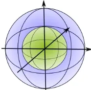
However, finding all neighbors at a large scale will require a large numberk, respectively a large search radius, such thatkD-trees become computationally demanding, too. To further accelerate processing it has been proposed to approximate larger neighbor-hoods, by first downsampling the point cloud and then picking a proportionally smaller numberk of nearest neighbors as rep-resentatives (Brodu and Lague, 2012). Embedded in our multi-scale setting this leads to the following simple algorithm (Fig-ure 2):(i)generate a scale pyramid by repeatedly downsampling the point cloud with a voxel-grid filter; and(ii)compute features at each scale from a fixed, small numberkof nearest neighbors. The widely used voxel-grid filter proceeds by dividing the bound-ing volume into evenly spaced cubes (“voxels”) of a given size, and replacing the points inside a voxel by their centroid. The method is computationally efficient: the memory footprint is rel-atively small, because the data is sparse and only voxels con-taining at least one point must be stored; and parallelization over different voxels is straight-forward. Moreover, the filtering grad-ually evens out the point density by skipping points only in high-density regions, such that a constantkwill at high scale levels
Figure 2. Sampling a point cloud at different scales (denoted by colors) reveals different properties of the underlying surface – here different surface normals (colored arrows). Multi-scale fea-ture extraction therefore improves classification.
approximate a fixed search radius. As a side effect, the reduced variation in point density also makes radius search feasible. We will exploit this to generate height features (see Table 1), because kNN is not reliable for cylindrical neighborhoods. In our imple-mentation we choosek= 10, which proved to be a suitable value (Weinmann et al., 2015), set the smallest voxel spacing to2.5cm, and use9rounds of standard multiplicative downsampling with a factor of2from one level to the next. These settings ensure that the memory footprint is at most twice as large as that of the high-est resolution, and reach a maximum voxel size (point spacing) of6.4m. In terms of runtime, the benefit of approximating the multi-scale neighborhood is twofold. First, a smallkis sufficient to capture even long-range geometric context, while the approxi-mation of the true neighborhood with a small, but well-distributed subsample is acceptable for coarse long-range information. Sec-ond, repeated downsampling greatly reduces the total number nof points, hence the neighborhood search itself gets faster at coarse scales. We point out that, alternatively, one could also generate a similar multi-scale representation with octrees (Else-berg et al., 2013).
3.2 Feature extraction
In our application we face a purely geometric classification prob-lem. We avoid using color and/or intensity values, which, de-pending on the recording technology, are not always available; and often also unreliable due to lighting effects. Given a point
pand its neighborhoodP, we follow (Weinmann et al., 2013)
and use 3D features based on eigenvalues1 λ1 ≥λ2 ≥λ3 ≥0 and corresponding eigenvectorse1,e2,e3of the covariance ten-sorC = 1
k
P
i∈P(pi−p)(pi−p)⊤, wherePis the set ofk
nearest neighbors andp= medi∈P(pi)is its medoid.
Eigenval-ues are normalised to sum up to1, so as to increase robustness against changes in point density. We augment the original feature set with four additional features that help to identify crease edges and occlusion boundaries, namely the first and second order mo-ments of the point neighborhood around the eigenvectorse1and
e2. Finally, in order to better describe vertical and/or thin objects like lamp posts, traffic signs or tree trunks, we also compute three further features from the height values (z-coordinates) in upright, cylindrical neighborhoods. Table 1 gives a summary and formal definition of all features.
The local structure tensor is computed fromk = 10points (cur-rent point plus9neighbors) over9scale levels ranging from voxel size0.025×0.025×0.025m3to6.4×6.4×6.4m3. In total this amounts to144feature dimensions. Note, the downsampling only affects which neighbors are found, via thekD-trees. Every point in the original data is classified, but in regions of extremely high point density multiple points may fall into the same voxel already at2.5cm resolution, and thus have the same neighbors.
1
Sum λ1+λ2+λ3 Omnivariance (λ1·λ2·λ3)13 Eigenentropy −P3
i=1λi·ln(λi)
Anisotropy (λ1−λ3)/λ1
covariance Planarity (λ2−λ3)/λ1
Linearity (λ1−λ2)/λ1
Vertical range zmax−zmin
height Height below z−zmin
Height above zmax−z
Table 1. Our basic feature set consists of geometric features based on eigenvalues of the local structure tensor, moments around the corresponding eigenvectors, as well as features computed in ver-tical columns around the point.
3.2.1 Approximate 3D shape context. The above covariance-based features describe surface properties. However, for more complex objects they may be insufficient, especially near contour edges. We found that explicit contour features in some situa-tions improve classification. To encode contour information, if needed, we have also developed efficient variants ofShape Con-text 3D (SC3D)(Frome et al., 2004) andSignature of Histogram of Orientations (SHOT)(Tombari et al., 2010). SC3D and SHOT are histogram-based descriptors similar in spirit to the original shape context for images (Belongie et al., 2002). Both divide the surroundings of a point into multiple smaller (radial) bins, see Figure 3, and therefore require large neighborhoods to be effec-tive. The main difference is that SC3D fills a single histogram with vectors from the center to the neighbors, whereas SHOT consists of a set of histograms over the point-wise normals, taken separately per bin. We have tried both descriptors in their origi-nal versions, and found that computing them densely for a single laser scan of moderate size (≈ 106
points) takes multiple days on a good workstation. Moreover, it turned out that, except near contour edges, the original SHOT and SC3D did not add much extra information to our feature set, and were almost completely ignored during classifier training. We therefore first learn a binary classifier that predicts from the features of Table 1 which points lie on (or near) a contour (Hackel et al., 2016). Only points with high contour likelihood are then used to fill the descriptors. This turns out to make them more informative, and at the same time speeds up the computation.
Again, our scale pyramid (Section 3.1) greatly accelerates the feature extraction. We donot compute all bins with the same (highest) point density. Instead, only histogram counts inside the smallest radial shell are computed at the highest resolution, whereas counts for larger shells are computed from progressively coarser scales. As long as there are more than a handful of points in each bin, the approximation roughly corresponds to rescaling the bin counts of the original histograms as a function of the ra-dius, and still characterizes the point distributions well. We dub our fast variants approximate SHOT (A-SHOT) and approximate SC3D (A-SC3D). Even with the proposed approximation, com-puting either of these descriptors densely takes≈30 minutes for 3·107
points. As will be seen in Section 4., they only slightly im-prove the results, hence we recommend the additional descriptors only for applications that require maximum accuracy.
Figure 3. Histogram bins (shells are different colored spheres).
3.3 Classification and training
Given feature vectorsx, we learn a supervised classifier that pre-dicts conditional probabilitiesP(y|x)of different class labelsy. We use a Random Forest classifier, because it is straight-forward to parallelize, is directly applicable to multi-class problems, by construction delivers probabilities, and has been shown to yield good results in reasonable time on large point clouds (Chehata et al., 2009, Weinmann et al., 2015). Random Forest parameters are found by minimizing the generalization error via 5-fold cross validation. We find50trees, Gini index as splitting criterion, and tree depths≈ 30to be optimal parameters for our application. For our particular problem, the class frequencies in a certain scan do not necessarily represent the prior distribution over the class labels, because objects closer to the scanner have quadratically more samples per unit of area than those further away. This ef-fect is a function of the scene layout and the scanner viewpoint. It can lead to heavily biased class frequencies and thus has to be accounted for. We resolve the issue pragmatically, by down-sampling the training set to approximately uniform resolution. Besides better approximating the true class distributions, down-sampling has the side effect that labelled data from a larger area fits into memory, which improves generalization capability of the classifier.
For maximum efficiency at test time we also traverse the random forest after training and build a list of the used features. Features that are not used are subsequently not extracted from test data.2 In practice all covariance features are used, only if one adds also the A-SC3D or A-SHOT descriptors some histogram bins are not selected. Note that reducing the feature dimension for testing only influences computation time. Memory usage is not affected, because at test time we only need to store point coordinates and the precomputedkD-tree structure. Features are computed on the fly and not stored. For very large test sets it is straight-forward to additionally split the point cloud into smaller (volumetric) slices or tiles with only the minimum overlap required for feature com-putation (Weinmann et al., 2015).
4. EXPERIMENTS
For our evaluation, data from different recording technologies was classified. To compare to prior art, we use well-known data-bases from mobile mapping devices, namelyParis-Rue-Cassette and Paris-Rue-Madame. These point clouds were recorded in Paris using laser scanners mounted on cars (Serna et al., 2014, Vallet et al., 2015). Both datasets are processed with the same training and test sets as in (Weinmann et al., 2015), which consist of 1000 training samples per class and≈1.2·107
, respectively ≈ 2·107
test samples. Furthermore, we test our method on multiple terrestrial laser scans from locations throughout Europe
2
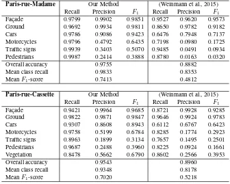
Paris-rue-Madame Our Method (Weinmann et al., 2015) Recall Precision F1 Recall Precision F1
Fac¸ade 0.9799 0.9902 0.9851 0.9527 0.9620 0.9573
Ground 0.9692 0.9934 0.9811 0.8650 0.9782 0.9182
Cars 0.9786 0.9086 0.9423 0.6476 0.7948 0.7137
Motorcycles 0.9796 0.4792 0.6435 0.7198 0.0980 0.1725
Traffic signs 0.9939 0.3403 0.5070 0.9485 0.0491 0.0934
Pedestrians 0.9987 0.2414 0.3888 0.8780 0.0163 0.0320
Overall accuracy 0.9755 0.8882
Mean class recall 0.9833 0.8353
MeanF1-score 0.7413 0.4812
Paris-rue-Cassette Our Method (Weinmann et al., 2015)
Recall Precision F1 Recall Precision F1
Fac¸ade 0.9421 0.9964 0.9685 0.8721 0.9928 0.9285
Ground 0.9822 0.9871 0.9847 0.9646 0.9924 0.9783
Cars 0.9307 0.8608 0.8943 0.6112 0.6767 0.6423
Motorcycles 0.9758 0.5199 0.6784 0.8285 0.1774 0.2923
Traffic signs 0.8963 0.1899 0.3134 0.7657 0.1495 0.2501
Pedestrians 0.9687 0.2488 0.3960 0.8225 0.0924 0.1661
Vegetation 0.8478 0.5662 0.6790 0.8602 0.2566 0.3953
Overall accuracy 0.9543 0.8960
Mean class recall 0.9348 0.8178
MeanF1-score 0.7020 0.5218
Table 2. Quantitative results for iQmulus / TerraMobilita and Paris-Rue-Madame databases.
and Asia. Each scan contains≈3·107
points and has been ac-quired from a single viewpoint, such that the data exhibits strong variations in point density. We learn the classifier from8scans (sub-sampled for training, see Section 3.3) and test on the other 10scans. On these more challenging examples we also evaluate the influence of the additional A-SHOT and A-SC3D descriptors. As performance metrics for quantitative evaluation, we use preci-sion,recallandF1-score, individually for each class. Moreover, we show overall accuracy and mean class recall over the whole dataset, to evaluate the overall performance.
4.1 Implementation Details
All software is implemented inC++, using thePoint Cloud Li-brary(pointclouds.org),FLANN(github.com/mariusmuja/ flann) for nearest-neighbor search and the ETH Random For-est Template Library(prs.igp.ethz.ch/research/Source_ code_and_datasets.html). All experiments are run on a stan-dard desktop PC with Intel Xeon E5-1650 CPU (hexa-core, 3.5 GHz) and 64 GB of RAM. The large amount of RAM is only needed for training, whereas classification of a typical point cloud requires<16GB. Point-wise classification is parallelized with OpenMP(openmp.org/wp) across the available CPU cores. In-tuitively, porting the classification part to the GPU should be straight-forward and could further reduce runtime.
Our classification routine consists of two computational stages. First, for each scale level thekD-tree structure is pre-computed. Second, the feature computation is run for each individual point, at each scale level (Section 3.2). During training, this is done for all points, so that all features are available for learning the classi-fier. The Random Forest uses Gini impurity as splitting criterion, its hyper-parameters (number and depth of trees) are found with grid search and 5-fold cross-validation. Typically, 50trees of maximum depth≈ 30are required. Having found the best pa-rameters, the classifier is relearned on the entire training set. At test time, the feature vector for each point is needed only once, hence features are not precomputed, but rather evaluated on the fly to save memory.
Paris-rue-Cassette (Weinmann et al., 2015) this paper
features 23,000 s 191 s
training 2 s 16 s
classification 90 s 60 s
total 23’092 s 267 s
Table 3. Computation times for processing the Paris-Rue-Cassette database an a single PC. Our feature computation is much faster. The comparison is indicative, implementation de-tails and hardware setup may differ, see text.
4.2 Results on Mobile Mapping Data
On the MLS datasets we can compare directly to previous work. The best results we are aware of are those of (Weinmann et al., 2015). Quantitative classification results with the base features (covariance, moment and height) are shown in Table 2. Our mean class recall is98.3% for Paris-Rue-Madame and93.5% for Paris-Rue-Cassette, while our overall accuracy is97.6%, respectively 95.4%. Most precision and recall values, as well as allF1-scores, are higher than the previously reported numbers. On average ourF1-scores are more than20% higher. We attribute the gains mainly to the fact that we need not restrict the number of scales, or select a single one, but instead supply the classifier with the full multi-scale pyramid from0.025to6.4m. The fact that prac-tically all features are used by the Random Forest supports this assertion. Moreover, the additional moment features, which are almost for free once the eigen-decomposition of the structure ten-sor has been done, seem to improve the performance near occlu-sion boundaries. Example views of the classified point clouds are depicted in Figure 4. A feature relevance test was performed by removing each feature in turn and re-training the classifier. The feature with the strongest individual influence isz−zminwith a
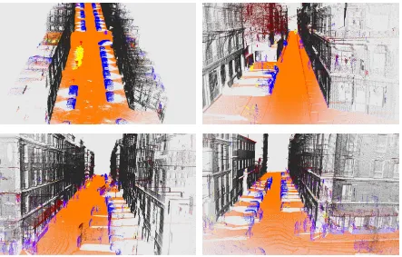
Figure 4. Results from iQmulus / TerraMobilita dataset.Top row:Paris-Rue-Madame (left) and Paris-Rue-Cassette (right) with classes: fac¸ade,ground,cars,motorcycles,traffic signs,pedestriansandvegetation.Bottom row:Further results without ground truth.
no ground truth, see Figure 4. Visually the method yields good results even though we do not use more training data, but stick with only1000training samples per class. Besides better accu-racy, our algorithm also greatly outperforms the baseline in terms of runtime, in spite of the higher-dimensional feature representa-tion. Our system is two orders of magnitude faster, see Table 3. We point out that the comparison should be seen as indicative: the timings for the baseline are those reported by the authors. Their software is also written inC++(called from Matlab). But it is single-threaded, and it was run on a different, albeit comparable, machine (64 GB RAM, Intel Core i7-3820 quad-core, 3.6 GHz).
4.3 Results on Terrestrial Laser Scans
The terrestrial laser scans are more challenging, for several rea-sons. The data was captured in both urban and rural environ-ments, so that there is more variety, and a greater degree of oc-clusion. Also, the training and testing datasets are from different physical locations, and constitute a stricter test of the classifier’s ability to generalize. Finally, the surveying-grade scanners used for recording have better angular resolution and higher range, leading to massive variations in point density between nearby and distant objects. There is also more data. The training data has≈500,000points, sampled from a total of2·108
points in the training scans. The test set has more than3·108
points. Table 4 shows that our proposed framework is able to cope rather well with the TLS data. Overall accuracy achieved with only base fea-tures is90.3%, at a mean class recall of79.7%. This results in 74.4%F1-score. Recall and precision values for the larger and easier classes are – as expected – lower than for the Paris, on the other hand the precision of smaller classes is significantly better, leading to a higher averageF1-score. The computation time for the complete test set is90minutes, including disk I/O.
These results can be further improved with additional histogram descriptors (Section 3.2.1), especially for thelow vegetationclass,
where the gains inF1-score reach8-9percent points. Overall, A-SC3D works a bit better than A-SHOT and is to be preferred. With the latter, classification of scanning artifacts on moving ob-jects is less reliable (−4percent points). However, the gains are rather small, at least for our class nomenclature, and they come at considerable computational cost. The following configuration gave the best trade-off between quality and speed: four shells with radii{1,2,4,16}m, 12 bins per shell, and4bins per local histogram of A-SHOT. With these settings the results improve for 6out of7classes, only forscanning artifactsthe additional de-scriptors potentially hurt performance. MeanF1-score goes up by1.7percent points. On the other hand, the feature computa-tion takes≈3×longer than for the base features, so adding A-SC3D or A-SHOT quadruples the processing time. Still, even large datasets with tens of millions of points are processed in less than one hour, which we consider acceptable for many ap-plications. Based on our results we do not generally recommend histogram-based descriptors, but note that they could have a sig-nificant impact for certain tasks and object classes.
5. CONCLUSION
We have described an efficient pipeline for point-wise classifica-tion of 3D point cloud data. The core of our method is an efficient strategy to construct approximate multi-scale neighborhoods in 3D point data. That scheme makes it possible to extract a rich feature representation in very little time, even in the presence of wildly varying point density. As a consequence, the proposed classification system outperforms the state of the art in terms of classification accuracy, while at the same time being fast enough for operational use on a single desktop machine.
Terrestrial Original Features Original Features + A-SHOT Original Features + A-SC3D Laser Scans Recall Precision F1 Recall Precision F1 Recall Precision F1 Man made terrain 0.8758 0.9433 0.9083 0.8757 0.9627 0.9171 0.8788 0.9651 0.9200 Natural terrain 0.8809 0.8921 0.8864 0.9064 0.8774 0.8916 0.9127 0.8747 0.8933 High vegetation 0.9129 0.8102 0.8585 0.8086 0.9254 0.8631 0.8655 0.8785 0.8720 Low vegetation 0.6496 0.4021 0.4967 0.6356 0.5364 0.5818 0.6685 0.5052 0.5755
Buildings 0.9592 0.9878 0.9733 0.9726 0.9813 0.9769 0.9676 0.9859 0.9766
Remaining hard scape 0.7879 0.4878 0.6025 0.8419 0.4743 0.6068 0.8256 0.4824 0.6090 Scanning artefacts 0.5127 0.4595 0.4847 0.3995 0.5039 0.4457 0.4197 0.5684 0.4829
Overall accuracy 0.9028 0.9097 0.9114
Mean class recall 0.7970 0.7772 0.7912
MeanF1-score 0.7443 0.7547 0.7613
Table 4. Quantitative results for terrestrial laser scans.
Figure 5. Results for terrestrial laser scans.Top row:urban street in St. Gallen (left), market square in Feldkirch (right). Bottom row: church in Bildstein (left), cathedral in St. Gallen (right) with classes:man-made terrain,natural terrain,high vegetation,low vegetation, buildings,remaining hard scapeandscanning artefacts.
one could try to explicitly detect and reconstruct line features to help in delineating the classes. Another possible direction is to sidestep feature design altogether and adapt the recently very successful deep neural networks to point clouds. The challenge here will be to remain efficient in the absence of a regular grid, al-though the voxel-grid neighborhoods built into our pipeline may provide a good starting point. Finally, on the technical level it would be interesting to port the method to the GPU to further improve speed.
REFERENCES
Belongie, S., Malik, J. and Puzicha, J., 2002. Shape matching and object recognition using shape contexts. IEEE TPAMI 24(4), pp. 509–522.
Blomley, R., Weinmann, M., Leitloff, J. and Jutzi, B., 2014. Shape distribution features for point cloud analysis-a geometric histogram approach on multiple scales. ISPRS Annals.
Boyko, A. and Funkhouser, T., 2011. Extracting roads from dense point clouds in large scale urban environment. ISPRS J Pho-togrammetry & Remote Sensing 66(6), pp. 2–12.
Brodu, N. and Lague, D., 2012. 3d terrestrial lidar data classifica-tion of complex natural scenes using a multi-scale dimensionality criterion: Applications in geomorphology. ISPRS J Photogram-metry & Remote Sensing 68, pp. 121–134.
Charaniya, A. P., Manduchi, R. and Lodha, S. K., 2004. Su-pervised parametric classification of aerial LiDAR data. CVPR Workshops.
Chehata, N., Guo, L. and Mallet, C., 2009. Airborne LiDAR feature selection for urban classification using random forests. ISPRS Archives.
Demantk´e, J., Mallet, C., David, N. and Vallet, B., 2011. Dimen-sionality based scale selection in 3d lidar point clouds. ISPRS Archives.
Dohan, D., Matejek, B. and Funkhouser, T., 2015. Learning Hi-erarchical Semantic Segmentation of LIDAR Data. International Conference on 3D Vision.
Elseberg, J., Borrmann, D. and N¨uchter, A., 2013. One billion points in the cloud–an octree for efficient processing of 3d laser scans. ISPRS J Photogrammetry & Remote Sensing 76, pp. 76– 88.
Friedman, J. H., Bentley, J. L. and Finkel, R. A., 1977. An al-gorithm for finding best matches in logarithmic expected time. ACM Transactions on Mathematical Software 3(3), pp. 209–226.
Frome, A., Huber, D., Kolluri, R., B¨ulow, T. and Malik, J., 2004. Recognizing objects in range data using regional point descrip-tors. ECCV.
Golovinskiy, A., Kim, V. G. and Funkhouser, T., 2009. Shape-based Recognition of 3D Point Clouds in Urban Environments. ICCV.
Haala, N., Brenner, C. and Anders, K.-H., 1998. 3d urban GIS from laser altimeter and 2d map data. ISPRS Archives.
Hackel, T., Wegner, J. D. and Schindler, K., 2016. Contour de-tection in unstructured 3d point clouds. CVPR.
He, K., Sun, J. and Tang, X., 2010. Guided image filtering. ECCV.
Hug, C. and Wehr, A., 1997. Detecting and identifying topo-graphic objects in imaging laser altimetry data. ISPRS Archives.
Johnson, A. and Hebert, M., 1999. Using spin images for efficient object recognition in cluttered 3d scenes. IEEE TPAMI 21(5), pp. 433–449.
Kim, E. and Medioni, G., 2011. Urban scene understanding from aerial and ground LIDAR data. Machine Vision and Applications 22, pp. 691–703.
Lafarge, F. and Mallet, C., 2012. Creating large-scale city models from 3d-point clouds: a robust approach with hybrid representa-tion. IJCV 99(1), pp. 69–85.
Lai, K., Bo, L. and Fox, D., 2014. Unsupervised feature learning for 3d scene labeling. ICRA.
Lalonde, J.-F., Vandapel, N., Huber, D. and Hebert, M., 2006. Natural terrain classification using three-dimensional ladar data for ground robot mobility. Journal of Field Robotics 23(1), pp. 839–861.
Li, Y., Wu, X., Chrysathou, Y., Sharf, A., Cohen-Or, D. and Mi-tra, N. J., 2011. Globfit: Consistently fitting primitives by dis-covering global relations. ACM Transactions on Graphics 30(4), pp. 52:1–52:12.
Maas, H.-G., 1999. The potential of height texture measures for the segmentation of airborne laserscanner data. International Airborne Remote Sensing Conference and Exhibition / Canadian Symposium on Remote Sensing.
Monnier, F., Vallet, B. and Soheilian, B., 2012. Trees detection from laser point clouds acquired in dense urban areas by a mobile mapping system. ISPRS Annals.
Muja, M. and Lowe, D. G., 2009. Fast approximate nearest neigh-bors with automatic algorithm configuration. VISAPP.
Najafi, M., Namin, S. T., Salzmann, M. and Petersson, L., 2014. Non-associative Higher-Order Markov Networks for Point Cloud Classification. ECCV.
Niemeyer, J., Wegner, J. D., Mallet, C., Rottensteiner, F. and So-ergel, U., 2011. Conditional Random Fields for Urban Scene Classification with Full Waveform LiDAR Data. Photogrammet-ric Image Analysis.
Orka, H. O., Naesset, E. and Bollandsas, O. M., 2012. Classify-ing species of individual trees by intensity and structure features derived from airborne laser scanner data. Remote Sensing of En-vironment 123, pp. 258–270.
Pauly, M., Keiser, R. and Gross, M., 2003. Multi-scale feature extraction on point-sampled surfaces. Computer Graphics Forum 22(3), pp. 281–289.
Pu, S. and Vosselman, G., 2009. Knowledge based reconstruction of building models from terrestrial laser scanning data. ISPRS J Photogrammetry & Remote Sensing 64, pp. 575–584.
Pu, S., Rutzinger, M., Vosselman, G. and Oude Elberink, S., 2011. Recognizing basic structures from mobile laser scanning data for road inventory studies. ISPRS J Photogrammetry & Re-mote Sensing 66, pp. 28–39.
Rottensteiner, F. and Briese, C., 2002. A new method for build-ing extraction in urban areas from high-resolution LIDAR data. ISPRS Archives.
Rusu, R., Holzbach, A., Blodow, N. and Beetz, M., 2009. Fast geometric point labeling using conditional random fields. IROS.
Schmidt, A., Niemeyer, J., Rottensteiner, F. and Soergel, U., 2014. Contextual Classification of Full Waveform Lidar Data in the Wadden Sea. IEEE Geoscience and Remote Sensing Letters 11(9), pp. 1614–1618.
Schnabel, R., Wahl, R. and Klein, R., 2007. Efficient RANSAC for point-cloud shape detection. Computer Graphics Forum 26(2), pp. 214–226.
Serna, A., Marcotegui, B., Goulette, F. and Deschaud, J.-E., 2014. Paris-rue-madame database: a 3d mobile laser scanner dataset for benchmarking urban detection, segmentation and clas-sification methods. ICPRAM.
Shapovalov, R., Velizhev, A. and Barinova, O., 2010. Non-associative markov networks for 3D point cloud classification. ISPRS Archives.
Tombari, F., Salti, S. and Di Stefano, L., 2010. Unique signatures of histograms for local surface description. ECCV.
Vallet, B., Br´edif, M., Serna, A., Marcotegui, B. and Paparodi-tis, N., 2015. Terramobilita/iqmulus urban point cloud analysis benchmark. Computers & Graphics 49, pp. 126–133.
Vosselman, G., Gorte, B., Sithole, G. and Rabbani, T., 2004. Rec-ognizing structure in laser scanner point clouds. ISPRS Archives.
Weinmann, M., Jutzi, B. and Mallet, C., 2013. Feature relevance assessment for the semantic interpretation of 3d point cloud data. ISPRS Annals.
Weinmann, M., Urban, S., Hinz, S., Jutzi, B. and Mallet, C., 2015. Distinctive 2d and 3d features for automated large-scale scene analysis in urban areas. Computers & Graphics 49, pp. 47– 57.
Wu, Z., Song, S., Khosla, A., Yu, F., Zhang, L., Tang, X. and Xiao, J., 2015. 3D ShapeNets: A deep representation for volu-metric shape modeling. CVPR.
Xiao, J. and Furukawa, Y., 2014. Reconstructing the world’s mu-seums. IJCV 110(3), pp. 243–258.